1. Introduction
1.1 Preface
本系列博文是和鲸社区的活动《20天吃掉那只PyTorch》学习的笔记,本篇为系列笔记的第六篇——
Pytorch 的高阶 API。该专栏是
Github 上 2.8K
星的项目,在学习该书的过程中可以参考阅读《Python深度学习》一书的第一部分"深度学习基础"内容。
《Python深度学习》这本书是 Keras 之父
Francois Chollet
所著,该书假定读者无任何机器学习知识,以Keras
为工具,使用丰富的范例示范深度学习的最佳实践,该书通俗易懂,全书没有一个数学公式,注重培养读者的深度学习直觉。
《Python深度学习》一书的第一部分的 4
个章节内容如下,预计读者可以在 20 小时之内学完。
- 什么是深度学习
- 神经网络的数学基础
- 神经网络入门
- 机器学习基础
本系列博文的大纲如下:
- 一、PyTorch的建模流程
- 二、PyTorch的核心概念
- 三、PyTorch的层次结构
- 四、PyTorch的低阶API
- 五、PyTorch的中阶API
- 六、PyTorch的高阶API
最后,本博文提供所使用的全部数据,读者可以从下述连接中下载数据:
1.2 Pytorch的高阶API
Pytorch 没有官方的高阶 API。一般通过
nn.Module 来构建模型并编写自定义训练循环。
为了更加方便地训练模型,本书的作者编写了仿 keras 的
Pytorch 模型接口:torchkeras, 作为
Pytorch 的高阶 API。
本章我们主要详细介绍 Pytorch 的高阶 API
如下相关的内容。
- 构建模型的3种方法(继承
nn.Module基类,使用nn.Sequential,辅助应用模型容器) - 训练模型的3种方法(脚本风格,函数风格,
torchkeras.Model类风格) - 使用
GPU训练模型(单GPU训练,多GPU训练)
2. 构建模型的3种方法
可以使用以下3种方式构建模型:
继承
nn.Module基类构建自定义模型。使用
nn.Sequential按层顺序构建模型。继承
nn.Module基类构建模型并辅助应用模型容器进行封装(nn.Sequential,nn.ModuleList,nn.ModuleDict)。
其中 第 1 种方式最为常见,第 2
种方式最简单,第 3 种方式最为灵活也较为复杂。推荐使用第
1 种方式构建模型。
1 | import torch |
2.1 继承nn.Module基类构建自定义模型
以下是继承 nn.Module
基类构建自定义模型的一个范例。模型中的用到的层一般在__init__
函数中定义,然后在 forward
方法中定义模型的正向传播逻辑。
1 | class Net(nn.Module): |
Results:
1 | Net( |
1 | summary(net,input_shape= (3,32,32)) |
Results:
1 | ---------------------------------------------------------------- |
2.2 使用nn.Sequential按层顺序构建模型
使用 nn.Sequential 按层顺序构建模型无需定义
forward 方法。仅仅适合于简单的模型。
以下是使用 nn.Sequential 搭建模型的一些等价方法。
2.2.1 利用 add_module
方法
1 | net = nn.Sequential() |
Results:
1 | Sequential( |
2.2.2 利用变长参数
这种方式构建时不能给每个层指定名称。
1 | net = nn.Sequential( |
Results:
1 | Sequential( |
2.2.3 利用 OrderedDict
1 | from collections import OrderedDict |
Results:
1 | Sequential( |
1 | summary(net,input_shape= (3,32,32)) |
Results:
1 | ---------------------------------------------------------------- |
2.3 继承nn.Module基类构建模型
继承 nn.Module
基类构建模型并辅助应用模型容器进行封装。
当模型的结构比较复杂时,我们可以应用模型容器(nn.Sequential,
nn.ModuleList,
nn.ModuleDict)对模型的部分结构进行封装。这样做会让模型整体更加有层次感,有时候也能减少代码量。
Note:在下面的范例中我们每次仅仅使用一种模型容器,但实际上这些模型容器的使用是非常灵活的,可以在一个模型中任意组合任意嵌套使用。
2.3.1 nn.Sequential 作为模型容器
1 | class Net(nn.Module): |
Results:
1 | Net( |
2.3.2 nn.ModuleList 作为模型容器
注意下面中的 ModuleList 不能用 Python
中的列表代替。
1 | class Net(nn.Module): |
Results:
1 | Net( |
1 | summary(net,input_shape= (3,32,32)) |
Results:
1 | ---------------------------------------------------------------- |
2.3.3 nn.ModuleDict 作为模型容器
注意下面中的 ModuleDict 不能用 Python
中的字典代替。
1 | class Net(nn.Module): |
Results:
1 | Net( |
1 | summary(net,input_shape= (3,32,32)) |
Results:
1 | ---------------------------------------------------------------- |
3. 训练模型的3种方法
Pytorch
通常需要用户编写自定义训练循环,训练循环的代码风格因人而异。
有 3 类典型的训练循环代码风格:
- 脚本形式训练循环
- 函数形式训练循环
- 类形式训练循环
下面以 minist 数据集的分类模型的训练为例,演示这
3 种训练模型的风格。其中类形式训练循环我们会使用
torchkeras.Model 和 torchkeras.LightModel
这两种方法。
3.1 Prepare data
1 | import torch |
Results:
60000
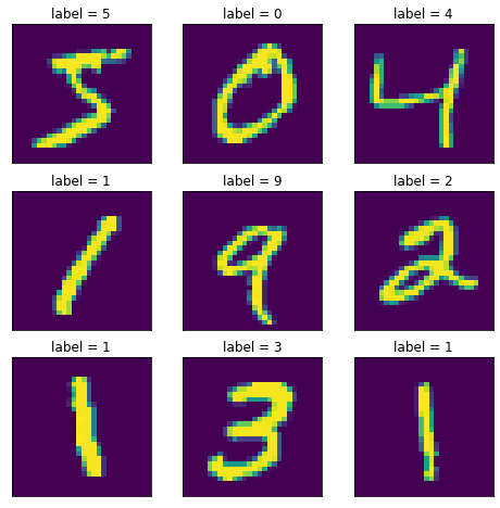
10000查看部分样本
1
2
3
4
5
6
7
8
9
10
11
12
13#查看部分样本
from matplotlib import pyplot as plt
plt.figure(figsize=(8,8))
for i in range(9):
img,label = ds_train[i]
img = torch.squeeze(img)
ax=plt.subplot(3,3,i+1)
ax.imshow(img.numpy())
ax.set_title("label = %d"%label)
ax.set_xticks([])
ax.set_yticks([])
plt.show()Results:
3.2 脚本风格
脚本风格的训练循环最为常见。
1 | net = nn.Sequential() |
Results:
1 | Sequential( |
1 | summary(net,input_shape=(1,32,32)) |
Results:
1 | ---------------------------------------------------------------- |
Model
1
2
3
4
5
6
7
8
9
10
11
12
13
14
15
16
17
18
19
20
21
22
23
24
25
26
27
28
29
30
31
32
33
34
35
36
37
38
39
40
41
42
43
44
45
46
47
48
49
50
51
52
53
54
55
56
57
58
59
60
61
62
63
64
65
66
67
68
69
70
71
72
73
74
75
76
77
78import datetime
import numpy as np
import pandas as pd
from sklearn.metrics import accuracy_score
def accuracy(y_pred,y_true):
y_pred_cls = torch.argmax(nn.Softmax(dim=1)(y_pred),dim=1).data
return accuracy_score(y_true,y_pred_cls)
loss_func = nn.CrossEntropyLoss()
optimizer = torch.optim.Adam(params=net.parameters(),lr = 0.01)
metric_func = accuracy
metric_name = "accuracy"
epochs = 3
log_step_freq = 100
dfhistory = pd.DataFrame(columns = ["epoch","loss",metric_name,"val_loss","val_"+metric_name])
print("Start Training...")
nowtime = datetime.datetime.now().strftime('%Y-%m-%d %H:%M:%S')
print("=========="*8 + "%s"%nowtime)
for epoch in range(1,epochs+1):
# 1,训练循环-------------------------------------------------
net.train()
loss_sum = 0.0
metric_sum = 0.0
step = 1
for step, (features,labels) in enumerate(dl_train, 1):
# 梯度清零
optimizer.zero_grad()
# 正向传播求损失
predictions = net(features)
loss = loss_func(predictions,labels)
metric = metric_func(predictions,labels)
# 反向传播求梯度
loss.backward()
optimizer.step()
# 打印batch级别日志
loss_sum += loss.item()
metric_sum += metric.item()
if step%log_step_freq == 0:
print(("[step = %d] loss: %.3f, "+metric_name+": %.3f") %
(step, loss_sum/step, metric_sum/step))
# 2,验证循环-------------------------------------------------
net.eval()
val_loss_sum = 0.0
val_metric_sum = 0.0
val_step = 1
for val_step, (features,labels) in enumerate(dl_valid, 1):
with torch.no_grad():
predictions = net(features)
val_loss = loss_func(predictions,labels)
val_metric = metric_func(predictions,labels)
val_loss_sum += val_loss.item()
val_metric_sum += val_metric.item()
# 3,记录日志-------------------------------------------------
info = (epoch, loss_sum/step, metric_sum/step,
val_loss_sum/val_step, val_metric_sum/val_step)
dfhistory.loc[epoch-1] = info
# 打印epoch级别日志
print(("\nEPOCH = %d, loss = %.3f,"+ metric_name + \
" = %.3f, val_loss = %.3f, "+"val_"+ metric_name+" = %.3f")
%info)
nowtime = datetime.datetime.now().strftime('%Y-%m-%d %H:%M:%S')
print("\n"+"=========="*8 + "%s"%nowtime)
print('Finished Training...')Results:
1
2
3
4
5
6
7
8
9
10
11
12
13
14
15
16
17
18
19
20
21
22
23
24
25
26
27
28Start Training...
================================================================================2022-02-07 19:51:52
[step = 100] loss: 0.625, accuracy: 0.800
[step = 200] loss: 0.398, accuracy: 0.874
[step = 300] loss: 0.314, accuracy: 0.902
[step = 400] loss: 0.267, accuracy: 0.917
EPOCH = 1, loss = 0.244,accuracy = 0.924, val_loss = 0.105, val_accuracy = 0.968
================================================================================2022-02-07 19:52:59
[step = 100] loss: 0.109, accuracy: 0.966
[step = 200] loss: 0.112, accuracy: 0.966
[step = 300] loss: 0.110, accuracy: 0.966
[step = 400] loss: 0.106, accuracy: 0.968
EPOCH = 2, loss = 0.104,accuracy = 0.969, val_loss = 0.063, val_accuracy = 0.981
================================================================================2022-02-07 19:53:59
[step = 100] loss: 0.083, accuracy: 0.974
[step = 200] loss: 0.085, accuracy: 0.974
[step = 300] loss: 0.085, accuracy: 0.974
[step = 400] loss: 0.090, accuracy: 0.973
EPOCH = 3, loss = 0.090,accuracy = 0.973, val_loss = 0.063, val_accuracy = 0.983
================================================================================2022-02-07 19:55:01
Finished Training...
3.3 函数风格
该风格在脚本形式上作了简单的函数封装。
1 | class Net(nn.Module): |
Results:
1 | Net( |
1 | summary(net,input_shape=(1,32,32)) |
Results:
1 | ---------------------------------------------------------------- |
Model-Train_step
1
2
3
4
5
6
7
8
9
10
11
12
13
14
15
16
17
18
19
20
21
22
23
24
25
26
27
28
29
30
31
32
33
34
35
36
37
38
39
40
41
42
43
44
45
46
47
48import datetime
import numpy as np
import pandas as pd
from sklearn.metrics import accuracy_score
def accuracy(y_pred,y_true):
y_pred_cls = torch.argmax(nn.Softmax(dim=1)(y_pred),dim=1).data
return accuracy_score(y_true,y_pred_cls)
model = net
model.optimizer = torch.optim.SGD(model.parameters(),lr = 0.01)
model.loss_func = nn.CrossEntropyLoss()
model.metric_func = accuracy
model.metric_name = "accuracy"
def train_step(model,features,labels):
# 训练模式,dropout层发生作用
model.train()
# 梯度清零
model.optimizer.zero_grad()
# 正向传播求损失
predictions = model(features)
loss = model.loss_func(predictions,labels)
metric = model.metric_func(predictions,labels)
# 反向传播求梯度
loss.backward()
model.optimizer.step()
return loss.item(),metric.item()
def valid_step(model,features,labels):
# 预测模式,dropout层不发生作用
model.eval()
predictions = model(features)
loss = model.loss_func(predictions,labels)
metric = model.metric_func(predictions,labels)
return loss.item(), metric.item()
# 测试train_step效果
features,labels = next(iter(dl_train))
train_step(model,features,labels)Results:
(2.3197388648986816, 0.09375)Model-Train_model
1
2
3
4
5
6
7
8
9
10
11
12
13
14
15
16
17
18
19
20
21
22
23
24
25
26
27
28
29
30
31
32
33
34
35
36
37
38
39
40
41
42
43
44
45
46
47
48
49
50
51
52
53
54def train_model(model,epochs,dl_train,dl_valid,log_step_freq):
metric_name = model.metric_name
dfhistory = pd.DataFrame(columns = ["epoch","loss",metric_name,"val_loss","val_"+metric_name])
print("Start Training...")
nowtime = datetime.datetime.now().strftime('%Y-%m-%d %H:%M:%S')
print("=========="*8 + "%s"%nowtime)
for epoch in range(1,epochs+1):
# 1,训练循环-------------------------------------------------
loss_sum = 0.0
metric_sum = 0.0
step = 1
for step, (features,labels) in enumerate(dl_train, 1):
loss,metric = train_step(model,features,labels)
# 打印batch级别日志
loss_sum += loss
metric_sum += metric
if step%log_step_freq == 0:
print(("[step = %d] loss: %.3f, "+metric_name+": %.3f") %
(step, loss_sum/step, metric_sum/step))
# 2,验证循环-------------------------------------------------
val_loss_sum = 0.0
val_metric_sum = 0.0
val_step = 1
for val_step, (features,labels) in enumerate(dl_valid, 1):
val_loss,val_metric = valid_step(model,features,labels)
val_loss_sum += val_loss
val_metric_sum += val_metric
# 3,记录日志-------------------------------------------------
info = (epoch, loss_sum/step, metric_sum/step,
val_loss_sum/val_step, val_metric_sum/val_step)
dfhistory.loc[epoch-1] = info
# 打印epoch级别日志
print(("\nEPOCH = %d, loss = %.3f,"+ metric_name + \
" = %.3f, val_loss = %.3f, "+"val_"+ metric_name+" = %.3f")
%info)
nowtime = datetime.datetime.now().strftime('%Y-%m-%d %H:%M:%S')
print("\n"+"=========="*8 + "%s"%nowtime)
print('Finished Training...')
return dfhistory
epochs = 3
dfhistory = train_model(model,epochs,dl_train,dl_valid,log_step_freq = 100)Results:
1
2
3
4
5
6
7
8
9
10
11
12
13
14
15
16
17
18
19
20
21
22
23
24
25
26
27Start Training...
================================================================================2022-02-07 19:55:04
[step = 100] loss: 2.301, accuracy: 0.111
[step = 200] loss: 2.292, accuracy: 0.131
[step = 300] loss: 2.284, accuracy: 0.153
[step = 400] loss: 2.274, accuracy: 0.181
EPOCH = 1, loss = 2.266,accuracy = 0.206, val_loss = 2.201, val_accuracy = 0.421
================================================================================2022-02-07 19:56:02
[step = 100] loss: 2.185, accuracy: 0.411
[step = 200] loss: 2.153, accuracy: 0.434
[step = 300] loss: 2.110, accuracy: 0.454
[step = 400] loss: 2.046, accuracy: 0.472
EPOCH = 2, loss = 1.994,accuracy = 0.483, val_loss = 1.559, val_accuracy = 0.684
================================================================================2022-02-07 19:57:04
[step = 100] loss: 1.487, accuracy: 0.603
[step = 200] loss: 1.387, accuracy: 0.622
[step = 300] loss: 1.293, accuracy: 0.643
[step = 400] loss: 1.212, accuracy: 0.663
EPOCH = 3, loss = 1.158,accuracy = 0.678, val_loss = 0.696, val_accuracy = 0.854
================================================================================2022-02-07 19:57:59
Finished Training...
3.4 类风格 torchkeras.Model
此处使用 torchkeras.Model 构建模型,并调用
compile 方法和 fit
方法训练模型。使用该形式训练模型非常简洁明了。
1 | import torchkeras |
Results:
1 | Model( |
1 | model.summary(input_shape=(1,32,32)) |
Results:
1 | ---------------------------------------------------------------- |
Model
1
2
3
4
5
6
7
8
9
10
11from sklearn.metrics import accuracy_score
def accuracy(y_pred,y_true):
y_pred_cls = torch.argmax(nn.Softmax(dim=1)(y_pred),dim=1).data
return accuracy_score(y_true.numpy(),y_pred_cls.numpy())
model.compile(loss_func = nn.CrossEntropyLoss(),
optimizer= torch.optim.Adam(model.parameters(),lr = 0.02),
metrics_dict={"accuracy":accuracy})
dfhistory = model.fit(3,dl_train = dl_train, dl_val=dl_valid, log_step_freq=100)Results:
1
2
3
4
5
6
7
8
9
10
11
12
13
14
15
16
17
18
19
20
21
22
23
24
25
26
27
28
29
30
31
32
33
34
35
36
37
38
39
40Start Training ...
================================================================================2022-02-07 19:57:59
{'step': 100, 'loss': 1.004, 'accuracy': 0.653}
{'step': 200, 'loss': 0.631, 'accuracy': 0.787}
{'step': 300, 'loss': 0.49, 'accuracy': 0.837}
{'step': 400, 'loss': 0.417, 'accuracy': 0.863}
+-------+-------+----------+----------+--------------+
| epoch | loss | accuracy | val_loss | val_accuracy |
+-------+-------+----------+----------+--------------+
| 1 | 0.387 | 0.874 | 0.142 | 0.957 |
+-------+-------+----------+----------+--------------+
================================================================================2022-02-07 19:58:54
{'step': 100, 'loss': 0.162, 'accuracy': 0.95}
{'step': 200, 'loss': 0.169, 'accuracy': 0.95}
{'step': 300, 'loss': 0.162, 'accuracy': 0.952}
{'step': 400, 'loss': 0.157, 'accuracy': 0.953}
+-------+------+----------+----------+--------------+
| epoch | loss | accuracy | val_loss | val_accuracy |
+-------+------+----------+----------+--------------+
| 2 | 0.16 | 0.953 | 0.111 | 0.971 |
+-------+------+----------+----------+--------------+
================================================================================2022-02-07 19:59:50
{'step': 100, 'loss': 0.145, 'accuracy': 0.959}
{'step': 200, 'loss': 0.16, 'accuracy': 0.954}
{'step': 300, 'loss': 0.161, 'accuracy': 0.954}
{'step': 400, 'loss': 0.164, 'accuracy': 0.954}
+-------+-------+----------+----------+--------------+
| epoch | loss | accuracy | val_loss | val_accuracy |
+-------+-------+----------+----------+--------------+
| 3 | 0.161 | 0.955 | 0.132 | 0.965 |
+-------+-------+----------+----------+--------------+
================================================================================2022-02-07 20:00:51
Finished Training...
3.5 类风格 torchkeras.LightModel
下面示范 torchkeras.LightModel
的使用范例,详细用法可以参照
1 | import torchkeras |
Results:
1 | Global seed set to 1234 |
1 | ckpt_cb = pl.callbacks.ModelCheckpoint(monitor='val_loss') |
Results:
1 | GPU available: False, used: False |
4. 使用GPU训练模型
深度学习的训练过程常常非常耗时,一个模型训练几个小时是家常便饭,训练几天也是常有的事情,有时候甚至要训练几十天。
训练过程的耗时主要来自于两个部分,一部分来自 数据准备,另一部分来自 参数迭代。
数据准备
当数据准备过程还是模型训练时间的主要瓶颈时,我们可以使用更多进程来准备数据。
参数迭代
当参数迭代过程成为训练时间的主要瓶颈时,我们通常的方法是应用GPU来进行加速。
Pytorch 中使用 GPU
加速模型非常简单,只要将模型和数据移动到 GPU
上。核心代码只有以下几行。
- 定义模型
1 | device = torch.device("cuda:0" if torch.cuda.is_available() else "cpu") |
- 训练模型
1 | features = features.to(device) # 移动数据到cuda |
如果要使用多个 GPU
训练模型,也非常简单。只需要在将模型设置为数据并行风格模型。则模型移动到
GPU 上之后,会在每一个 GPU
上拷贝一个副本,并把数据平分到各个 GPU 上进行训练。
4.1 GPU 相关基本操作
在 Colab 笔记本中:修改->笔记本设置->硬件加速器
中选择 GPU
注:以下代码只能在 Colab
上才能正确执行。可点击如下链接,直接在 colab
中运行范例代码。《torch使用gpu训练模型》:https://colab.research.google.com/drive/1FDmi44-U3TFRCt9MwGn4HIj2SaaWIjHu?usp=sharing
1 | import torch |
查看
gpu信息1
2
3
4
5
6# 1,查看gpu信息
if_cuda = torch.cuda.is_available()
print("if_cuda=",if_cuda)
gpu_count = torch.cuda.device_count()
print("gpu_count=",gpu_count)Resutls:
if_cuda= False gpu_count= 0将张量在
gpu和cpu间移动由于本机
gpu未正常配置,下述代码会报错。1
2
3
4
5
6
7
8# 2,将张量在gpu和cpu间移动
tensor = torch.rand((100,100))
tensor_gpu = tensor.to("cuda:0") # 或者 tensor_gpu = tensor.cuda()
print(tensor_gpu.device)
print(tensor_gpu.is_cuda)
tensor_cpu = tensor_gpu.to("cpu") # 或者 tensor_cpu = tensor_gpu.cpu()
print(tensor_cpu.device)Results:
1
2
3
4
5
6
7
8
9
10
11
12
13
14
15
16
17
18
19
20
21
22
23
24
25
26
27
28---------------------------------------------------------------------------
RuntimeError Traceback (most recent call last)
<ipython-input-24-cb760e986663> in <module>
1 # 2,将张量在gpu和cpu间移动
2 tensor = torch.rand((100,100))
----> 3 tensor_gpu = tensor.to("cuda:0") # 或者 tensor_gpu = tensor.cuda()
4 print(tensor_gpu.device)
5 print(tensor_gpu.is_cuda)
D:\Programs\Anaconda\lib\site-packages\torch\cuda\__init__.py in _lazy_init()
170 # This function throws if there's a driver initialization error, no GPUs
171 # are found or any other error occurs
--> 172 torch._C._cuda_init()
173 # Some of the queued calls may reentrantly call _lazy_init();
174 # we need to just return without initializing in that case.
RuntimeError: CUDA driver initialization failed, you might not have a CUDA gpu.
3. 将模型中的全部张量移动到gpu上
```python
# 3,将模型中的全部张量移动到gpu上
net = nn.Linear(2,1)
print(next(net.parameters()).is_cuda)
net.to("cuda:0") # 将模型中的全部参数张量依次到GPU上,注意,无需重新赋值为 net = net.to("cuda:0")
print(next(net.parameters()).is_cuda)
print(next(net.parameters()).device)Results:
1
2
3
4
5
6
7
8
9
10
11
12
13
14
15
16
17
18
19
20
21
22
23
24
25
26
27
28
29
30
31
32
33
34
35
36
37
38
39
40False
---------------------------------------------------------------------------
RuntimeError Traceback (most recent call last)
<ipython-input-25-f51cc87d7898> in <module>
2 net = nn.Linear(2,1)
3 print(next(net.parameters()).is_cuda)
----> 4 net.to("cuda:0") # 将模型中的全部参数张量依次到GPU上,注意,无需重新赋值为 net = net.to("cuda:0")
5 print(next(net.parameters()).is_cuda)
6 print(next(net.parameters()).device)
D:\Programs\Anaconda\lib\site-packages\torch\nn\modules\module.py in to(self, *args, **kwargs)
850 return t.to(device, dtype if t.is_floating_point() or t.is_complex() else None, non_blocking)
851
--> 852 return self._apply(convert)
853
854 def register_backward_hook(
D:\Programs\Anaconda\lib\site-packages\torch\nn\modules\module.py in _apply(self, fn)
550 # `with torch.no_grad():`
551 with torch.no_grad():
--> 552 param_applied = fn(param)
553 should_use_set_data = compute_should_use_set_data(param, param_applied)
554 if should_use_set_data:
D:\Programs\Anaconda\lib\site-packages\torch\nn\modules\module.py in convert(t)
848 return t.to(device, dtype if t.is_floating_point() or t.is_complex() else None,
849 non_blocking, memory_format=convert_to_format)
--> 850 return t.to(device, dtype if t.is_floating_point() or t.is_complex() else None, non_blocking)
851
852 return self._apply(convert)
D:\Programs\Anaconda\lib\site-packages\torch\cuda\__init__.py in _lazy_init()
170 # This function throws if there's a driver initialization error, no GPUs
171 # are found or any other error occurs
--> 172 torch._C._cuda_init()
173 # Some of the queued calls may reentrantly call _lazy_init();
174 # we need to just return without initializing in that case.
RuntimeError: CUDA driver initialization failed, you might not have a CUDA gpu.创建支持多个gpu数据并行的模型
1
2
3
4
5
6
7
8
9
10
11
12
13# 4,创建支持多个gpu数据并行的模型
linear = nn.Linear(2,1)
print(next(linear.parameters()).device)
model = nn.DataParallel(linear)
print(model.device_ids)
print(next(model.module.parameters()).device)
#注意保存参数时要指定保存model.module的参数
torch.save(model.module.state_dict(), data_dir + "model_parameter.pkl")
linear = nn.Linear(2,1)
linear.load_state_dict(torch.load(data_dir + "model_parameter.pkl"))Results:
1
2
3
4
5cpu
[]
cpu
<All keys matched successfully>清空
cuda缓存1
2
3
4# 5,清空cuda缓存
# 该方法在cuda超内存时十分有用
torch.cuda.empty_cache()
4.2 矩阵乘法范例
下面分别使用 CPU 和 GPU
作一个矩阵乘法,并比较其计算效率。
1 | import time |
使用
cpu1
2
3
4
5
6
7
8
9
10# 使用cpu
a = torch.rand((10000,200))
b = torch.rand((200,10000))
tic = time.time()
c = torch.matmul(a,b)
toc = time.time()
print(toc-tic)
print(a.device)
print(b.device)Results:
0.6119661331176758 cpu cpu使用
gpu1
2
3
4
5
6
7
8
9
10
11# 使用gpu
device = torch.device("cuda:0" if torch.cuda.is_available() else "cpu")
a = torch.rand((10000,200),device = device) #可以指定在GPU上创建张量
b = torch.rand((200,10000)) #也可以在CPU上创建张量后移动到GPU上
b = b.to(device) #或者 b = b.cuda() if torch.cuda.is_available() else b
tic = time.time()
c = torch.matmul(a,b)
toc = time.time()
print(toc-tic)
print(a.device)
print(b.device)Results:
0.43799781799316406 cpu cpu
4.3 线性回归范例
下面对比使用 CPU 和 GPU
训练一个线性回归模型的效率
4.3.1 使用CPU
Prepare data
1
2
3
4
5
6
7# 准备数据
n = 1000000 #样本数量
X = 10*torch.rand([n,2])-5.0 #torch.rand是均匀分布
w0 = torch.tensor([[2.0,-3.0]])
b0 = torch.tensor([[10.0]])
Y = X@w0.t() + b0 + torch.normal( 0.0,2.0,size = [n,1]) # @表示矩阵乘法,增加正态扰动Define model
1
2
3
4
5
6
7
8
9
10
11# 定义模型
class LinearRegression(nn.Module):
def __init__(self):
super().__init__()
self.w = nn.Parameter(torch.randn_like(w0))
self.b = nn.Parameter(torch.zeros_like(b0))
#正向传播
def forward(self,x):
return x@self.w.t() + self.b
linear = LinearRegression()Train model
1
2
3
4
5
6
7
8
9
10
11
12
13
14
15
16
17
18# 训练模型
optimizer = torch.optim.Adam(linear.parameters(),lr = 0.1)
loss_func = nn.MSELoss()
def train(epoches):
tic = time.time()
for epoch in range(epoches):
optimizer.zero_grad()
Y_pred = linear(X)
loss = loss_func(Y_pred,Y)
loss.backward()
optimizer.step()
if epoch%50==0:
print({"epoch":epoch,"loss":loss.item()})
toc = time.time()
print("time used:",toc-tic)
train(500)Results:
1
2
3
4
5
6
7
8
9
10
11{'epoch': 0, 'loss': 3.998589515686035}
{'epoch': 50, 'loss': 3.9990580081939697}
{'epoch': 100, 'loss': 3.998594045639038}
{'epoch': 150, 'loss': 3.998589515686035}
{'epoch': 200, 'loss': 3.998589515686035}
{'epoch': 250, 'loss': 3.998589515686035}
{'epoch': 300, 'loss': 3.998589277267456}
{'epoch': 350, 'loss': 3.998589515686035}
{'epoch': 400, 'loss': 3.998589515686035}
{'epoch': 450, 'loss': 3.998589515686035}
time used: 11.279652833938599
4.3.2 使用 gpu
Note:由于本机未正常跑配置
gpu,因此使用 cpu
跑通,代码逻辑无问题。若想复现代码,直接使用下述代码即可。
Prepare data
1
2
3
4
5
6
7
8
9
10
11
12# 准备数据
n = 1000000 #样本数量
X = 10*torch.rand([n,2])-5.0 #torch.rand是均匀分布
w0 = torch.tensor([[2.0,-3.0]])
b0 = torch.tensor([[10.0]])
Y = X@w0.t() + b0 + torch.normal( 0.0,2.0,size = [n,1]) # @表示矩阵乘法,增加正态扰动
# 移动到GPU上
print("torch.cuda.is_available() = ", torch.cuda.is_available())
X = X.cuda()
Y = Y.cuda()
print("X.device:",X.device)
print("Y.device:",Y.device)Results:
1
2
3torch.cuda.is_available() = False
X.device: cpu
Y.device: cpuDefine model
1
2
3
4
5
6
7
8
9
10
11
12
13
14
15
16
17
18# 定义模型
class LinearRegression(nn.Module):
def __init__(self):
super().__init__()
self.w = nn.Parameter(torch.randn_like(w0))
self.b = nn.Parameter(torch.zeros_like(b0))
#正向传播
def forward(self,x):
return x@self.w.t() + self.b
linear = LinearRegression()
# 移动模型到GPU上
device = torch.device("cuda:0" if torch.cuda.is_available() else "cpu")
linear.to(device)
#查看模型是否已经移动到GPU上
print("if on cuda:",next(linear.parameters()).is_cuda)Results:
if on cuda: FalseTrain model
1
2
3
4
5
6
7
8
9
10
11
12
13
14
15
16
17
18# 训练模型
optimizer = torch.optim.Adam(linear.parameters(),lr = 0.1)
loss_func = nn.MSELoss()
def train(epoches):
tic = time.time()
for epoch in range(epoches):
optimizer.zero_grad()
Y_pred = linear(X)
loss = loss_func(Y_pred,Y)
loss.backward()
optimizer.step()
if epoch%50==0:
print({"epoch":epoch,"loss":loss.item()})
toc = time.time()
print("time used:",toc-tic)
train(500)Results:
1
2
3
4
5
6
7
8
9
10
11{'epoch': 0, 'loss': 185.2291717529297}
{'epoch': 50, 'loss': 33.15369415283203}
{'epoch': 100, 'loss': 9.041170120239258}
{'epoch': 150, 'loss': 4.488009929656982}
{'epoch': 200, 'loss': 4.019914150238037}
{'epoch': 250, 'loss': 3.9960811138153076}
{'epoch': 300, 'loss': 3.9955568313598633}
{'epoch': 350, 'loss': 3.995553493499756}
{'epoch': 400, 'loss': 3.995553493499756}
{'epoch': 450, 'loss': 3.995553493499756}
time used: 11.048993825912476
4.4 torchkeras.Model 使用单 GPU 范例
下面演示使用 torchkeras.Model 来应用 GPU
训练模型的方法。
其对应的CPU训练模型代码参见《6-2,训练模型的 3
种方法》,本例仅需要在它的基础上增加一行代码,在
model.compile 时指定 device 即可。
Prepare data
1
!pip install -U torchkeras
1
2
3
4
5
6
7
8
9
10
11
12
13
14
15
16
17
18import torch
from torch import nn
import torchvision
from torchvision import transforms
import torchkeras
transform = transforms.Compose([transforms.ToTensor()])
ds_train = torchvision.datasets.MNIST(root=data_dir + "minist/",train=True,download=True,transform=transform)
ds_valid = torchvision.datasets.MNIST(root=data_dir + "minist/",train=False,download=True,transform=transform)
dl_train = torch.utils.data.DataLoader(ds_train, batch_size=128, shuffle=True, num_workers=1)
dl_valid = torch.utils.data.DataLoader(ds_valid, batch_size=128, shuffle=False, num_workers=1)
print(len(ds_train))
print(len(ds_valid))Results:
60000 10000Note:上述代码中,
num_worders如果设置为4,会在模型训练过程中,报如下错误:1
RuntimeError: DataLoader worker (pid(s) 9320, 8476, 8504, 4600) exited unexpectedly
为了避免上述错误,在上述代码中将参数
num_workers设置为1。1
2
3
4
5
6
7
8
9
10
11
12
13#查看部分样本
from matplotlib import pyplot as plt
plt.figure(figsize=(8,8))
for i in range(9):
img,label = ds_train[i]
img = torch.squeeze(img)
ax=plt.subplot(3,3,i+1)
ax.imshow(img.numpy())
ax.set_title("label = %d"%label)
ax.set_xticks([])
ax.set_yticks([])
plt.show()Results:

Define model
1
2
3
4
5
6
7
8
9
10
11
12
13
14
15
16
17
18
19
20
21
22
23class CnnModel(nn.Module):
def __init__(self):
super().__init__()
self.layers = nn.ModuleList([
nn.Conv2d(in_channels=1,out_channels=32,kernel_size = 3),
nn.MaxPool2d(kernel_size = 2,stride = 2),
nn.Conv2d(in_channels=32,out_channels=64,kernel_size = 5),
nn.MaxPool2d(kernel_size = 2,stride = 2),
nn.Dropout2d(p = 0.1),
nn.AdaptiveMaxPool2d((1,1)),
nn.Flatten(),
nn.Linear(64,32),
nn.ReLU(),
nn.Linear(32,10)]
)
def forward(self,x):
for layer in self.layers:
x = layer(x)
return x
net = CnnModel()
model = torchkeras.Model(net)
model.summary(input_shape=(1,32,32))Results:
1
2
3
4
5
6
7
8
9
10
11
12
13
14
15
16
17
18
19
20
21
22
23----------------------------------------------------------------
Layer (type) Output Shape Param #
================================================================
Conv2d-1 [-1, 32, 30, 30] 320
MaxPool2d-2 [-1, 32, 15, 15] 0
Conv2d-3 [-1, 64, 11, 11] 51,264
MaxPool2d-4 [-1, 64, 5, 5] 0
Dropout2d-5 [-1, 64, 5, 5] 0
AdaptiveMaxPool2d-6 [-1, 64, 1, 1] 0
Flatten-7 [-1, 64] 0
Linear-8 [-1, 32] 2,080
ReLU-9 [-1, 32] 0
Linear-10 [-1, 10] 330
================================================================
Total params: 53,994
Trainable params: 53,994
Non-trainable params: 0
----------------------------------------------------------------
Input size (MB): 0.003906
Forward/backward pass size (MB): 0.359695
Params size (MB): 0.205971
Estimated Total Size (MB): 0.569572
----------------------------------------------------------------Train model
1
2
3
4
5
6
7
8
9
10
11
12
13
14from sklearn.metrics import accuracy_score
def accuracy(y_pred,y_true):
y_pred_cls = torch.argmax(nn.Softmax(dim=1)(y_pred),dim=1).data
return accuracy_score(y_true.cpu().numpy(),y_pred_cls.cpu().numpy())
# 注意此处要将数据先移动到cpu上,然后才能转换成numpy数组
device = torch.device("cuda:0" if torch.cuda.is_available() else "cpu")
model.compile(loss_func = nn.CrossEntropyLoss(),
optimizer= torch.optim.Adam(model.parameters(),lr = 0.02),
metrics_dict={"accuracy":accuracy},device = device) # 注意此处compile时指定了device
dfhistory = model.fit(3,dl_train = dl_train, dl_val=dl_valid, log_step_freq=100)Results:
1
2
3
4
5
6
7
8
9
10
11
12
13
14
15
16
17
18
19
20
21
22
23
24
25
26
27
28
29
30
31
32
33
34
35
36
37
38
39Start Training ...
================================================================================2022-02-07 20:25:25
{'step': 100, 'loss': 0.865, 'accuracy': 0.712}
{'step': 200, 'loss': 0.548, 'accuracy': 0.821}
{'step': 300, 'loss': 0.426, 'accuracy': 0.863}
{'step': 400, 'loss': 0.362, 'accuracy': 0.885}
+-------+-------+----------+----------+--------------+
| epoch | loss | accuracy | val_loss | val_accuracy |
+-------+-------+----------+----------+--------------+
| 1 | 0.333 | 0.895 | 0.092 | 0.973 |
+-------+-------+----------+----------+--------------+
================================================================================2022-02-07 20:26:24
{'step': 100, 'loss': 0.158, 'accuracy': 0.953}
{'step': 200, 'loss': 0.163, 'accuracy': 0.952}
{'step': 300, 'loss': 0.161, 'accuracy': 0.953}
{'step': 400, 'loss': 0.158, 'accuracy': 0.955}
+-------+-------+----------+----------+--------------+
| epoch | loss | accuracy | val_loss | val_accuracy |
+-------+-------+----------+----------+--------------+
| 2 | 0.154 | 0.956 | 0.13 | 0.964 |
+-------+-------+----------+----------+--------------+
================================================================================2022-02-07 20:27:20
{'step': 100, 'loss': 0.117, 'accuracy': 0.967}
{'step': 200, 'loss': 0.13, 'accuracy': 0.964}
{'step': 300, 'loss': 0.129, 'accuracy': 0.964}
{'step': 400, 'loss': 0.138, 'accuracy': 0.963}
+-------+-------+----------+----------+--------------+
| epoch | loss | accuracy | val_loss | val_accuracy |
+-------+-------+----------+----------+--------------+
| 3 | 0.142 | 0.962 | 0.108 | 0.973 |
+-------+-------+----------+----------+--------------+
================================================================================2022-02-07 20:28:18
Finished Training...Evaluate model
1
2
3
4
5
6
7
8
9
10
11
12
13
14
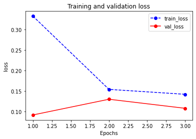
15import matplotlib.pyplot as plt
def plot_metric(dfhistory, metric):
train_metrics = dfhistory[metric]
val_metrics = dfhistory['val_'+metric]
epochs = range(1, len(train_metrics) + 1)
plt.plot(epochs, train_metrics, 'bo--')
plt.plot(epochs, val_metrics, 'ro-')
plt.title('Training and validation '+ metric)
plt.xlabel("Epochs")
plt.ylabel(metric)
plt.legend(["train_"+metric, 'val_'+metric])
plt.show()
plot_metric(dfhistory,"loss")Results:
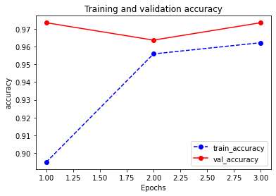
1
plot_metric(dfhistory,"accuracy")
Results:
Predict
1
model.predict(dl_valid)[0:10]
Results:
1
2
3
4
5
6
7
8
9
10
11
12
13
14
15
16
17
18
19
20tensor([[ -1.5347, 13.6357, 11.0183, -1.2204, 6.1134, -8.5289, -1.1970,
23.4888, -1.5858, 6.7930],
[ 5.7372, 6.6389, 21.1408, 8.8913, -8.1413, 1.0067, -0.5886,
7.1115, 3.5795, -5.1366],
[-10.7933, 32.6671, 6.6553, -9.0977, 5.0349, 3.5976, 0.2760,
4.0876, -0.5267, 0.7889],
[ 16.0825, 2.9832, 1.0242, -1.5304, 3.6435, -0.0766, 5.2385,
-1.9654, 5.8100, 4.1158],
[ -5.6585, 6.8265, 5.9029, -16.5844, 20.1805, -4.4995, 6.3734,
8.1729, -6.3171, 3.0607],
[-11.3707, 42.0231, 9.0211, -11.6561, 10.3878, 2.4693, 2.1876,
8.7440, -2.0002, 3.4919],
[ -3.1595, 3.6438, 3.2809, -9.1543, 11.1751, -2.1898, 3.0125,
4.4434, -3.1949, 1.9520],
[ 1.0515, -4.7944, 0.4023, 0.7020, 2.4049, -1.9072, -2.7254,
2.2177, 1.7448, 6.5435],
[ 0.6616, -1.2879, -0.6804, -2.7895, 0.9016, 7.1269, 2.9752,
0.0648, 0.6270, -0.4624],
[ 1.1252, -10.2878, -0.3109, 1.9929, 6.1019, -2.8175, -6.0583,
4.7262, 4.1898, 15.1963]])Save model
1
2
3
4
5
6
7
8
9
10
11# save the model parameters
torch.save(model.state_dict(), data_dir + "model_parameter.pkl")
model_clone = torchkeras.Model(CnnModel())
model_clone.load_state_dict(torch.load(data_dir + "model_parameter.pkl"))
model_clone.compile(loss_func = nn.CrossEntropyLoss(),
optimizer= torch.optim.Adam(model.parameters(),lr = 0.02),
metrics_dict={"accuracy":accuracy},device = device) # 注意此处compile时指定了device
model_clone.evaluate(dl_valid)Results:
{'val_loss': 0.10813457745549569, 'val_accuracy': 0.9733979430379747}
4.5. torchkeras.Model 使用多 GPU 范例
注:以下范例需要在有多个GPU的机器上跑。如果在单 GPU
的机器上跑,也能跑通,但是实际上使用的是单个 GPU。
Prepare data
1
2
3
4
5
6
7
8
9
10
11
12
13
14
15
16
17
18import torch
from torch import nn
import torchvision
from torchvision import transforms
import torchkeras
transform = transforms.Compose([transforms.ToTensor()])
ds_train = torchvision.datasets.MNIST(root= data_dir + "minist/",train=True,download=True,transform=transform)
ds_valid = torchvision.datasets.MNIST(root=data_dir + "minist/",train=False,download=True,transform=transform)
dl_train = torch.utils.data.DataLoader(ds_train, batch_size=128, shuffle=True, num_workers=1)
dl_valid = torch.utils.data.DataLoader(ds_valid, batch_size=128, shuffle=False, num_workers=1)
print(len(ds_train))
print(len(ds_valid))Results:
60000 10000Define model
1
2
3
4
5
6
7
8
9
10
11
12
13
14
15
16
17
18
19
20
21
22
23
24class CnnModule(nn.Module):
def __init__(self):
super().__init__()
self.layers = nn.ModuleList([
nn.Conv2d(in_channels=1,out_channels=32,kernel_size = 3),
nn.MaxPool2d(kernel_size = 2,stride = 2),
nn.Conv2d(in_channels=32,out_channels=64,kernel_size = 5),
nn.MaxPool2d(kernel_size = 2,stride = 2),
nn.Dropout2d(p = 0.1),
nn.AdaptiveMaxPool2d((1,1)),
nn.Flatten(),
nn.Linear(64,32),
nn.ReLU(),
nn.Linear(32,10)]
)
def forward(self,x):
for layer in self.layers:
x = layer(x)
return x
net = nn.DataParallel(CnnModule()) #Attention this line!!!
model = torchkeras.Model(net)
model.summary(input_shape=(1,32,32))Results:
1
2
3
4
5
6
7
8
9
10
11
12
13
14
15
16
17
18
19
20
21
22
23----------------------------------------------------------------
Layer (type) Output Shape Param #
================================================================
Conv2d-1 [-1, 32, 30, 30] 320
MaxPool2d-2 [-1, 32, 15, 15] 0
Conv2d-3 [-1, 64, 11, 11] 51,264
MaxPool2d-4 [-1, 64, 5, 5] 0
Dropout2d-5 [-1, 64, 5, 5] 0
AdaptiveMaxPool2d-6 [-1, 64, 1, 1] 0
Flatten-7 [-1, 64] 0
Linear-8 [-1, 32] 2,080
ReLU-9 [-1, 32] 0
Linear-10 [-1, 10] 330
================================================================
Total params: 53,994
Trainable params: 53,994
Non-trainable params: 0
----------------------------------------------------------------
Input size (MB): 0.003906
Forward/backward pass size (MB): 0.359695
Params size (MB): 0.205971
Estimated Total Size (MB): 0.569572
----------------------------------------------------------------Training model
1
2
3
4
5
6
7
8
9
10
11
12
13from sklearn.metrics import accuracy_score
def accuracy(y_pred,y_true):
y_pred_cls = torch.argmax(nn.Softmax(dim=1)(y_pred),dim=1).data
return accuracy_score(y_true.cpu().numpy(),y_pred_cls.cpu().numpy())
# 注意此处要将数据先移动到cpu上,然后才能转换成numpy数组
device = torch.device("cuda:0" if torch.cuda.is_available() else "cpu")
model.compile(loss_func = nn.CrossEntropyLoss(),
optimizer= torch.optim.Adam(model.parameters(),lr = 0.02),
metrics_dict={"accuracy":accuracy},device = device) # 注意此处compile时指定了device
dfhistory = model.fit(3,dl_train = dl_train, dl_val=dl_valid, log_step_freq=100)Results:
1
2
3
4
5
6
7
8
9
10
11
12
13
14
15
16
17
18
19
20
21
22
23
24
25
26
27
28
29
30
31
32
33
34
35
36
37
38
39Start Training ...
================================================================================2022-02-07 20:36:45
{'step': 100, 'loss': 0.919, 'accuracy': 0.683}
{'step': 200, 'loss': 0.57, 'accuracy': 0.808}
{'step': 300, 'loss': 0.442, 'accuracy': 0.853}
{'step': 400, 'loss': 0.381, 'accuracy': 0.876}
+-------+-------+----------+----------+--------------+
| epoch | loss | accuracy | val_loss | val_accuracy |
+-------+-------+----------+----------+--------------+
| 1 | 0.352 | 0.886 | 0.166 | 0.951 |
+-------+-------+----------+----------+--------------+
================================================================================2022-02-07 20:38:01
{'step': 100, 'loss': 0.157, 'accuracy': 0.956}
{'step': 200, 'loss': 0.146, 'accuracy': 0.958}
{'step': 300, 'loss': 0.144, 'accuracy': 0.959}
{'step': 400, 'loss': 0.146, 'accuracy': 0.958}
+-------+-------+----------+----------+--------------+
| epoch | loss | accuracy | val_loss | val_accuracy |
+-------+-------+----------+----------+--------------+
| 2 | 0.141 | 0.96 | 0.095 | 0.971 |
+-------+-------+----------+----------+--------------+
================================================================================2022-02-07 20:39:01
{'step': 100, 'loss': 0.109, 'accuracy': 0.969}
{'step': 200, 'loss': 0.139, 'accuracy': 0.963}
{'step': 300, 'loss': 0.147, 'accuracy': 0.962}
{'step': 400, 'loss': 0.144, 'accuracy': 0.963}
+-------+-------+----------+----------+--------------+
| epoch | loss | accuracy | val_loss | val_accuracy |
+-------+-------+----------+----------+--------------+
| 3 | 0.149 | 0.962 | 0.136 | 0.97 |
+-------+-------+----------+----------+--------------+
================================================================================2022-02-07 20:40:01
Finished Training...
- Evaluate model
1
2
3
4
5
6
7
8
9
10
11
12
13
14
15import matplotlib.pyplot as plt
def plot_metric(dfhistory, metric):
train_metrics = dfhistory[metric]
val_metrics = dfhistory['val_'+metric]
epochs = range(1, len(train_metrics) + 1)
plt.plot(epochs, train_metrics, 'bo--')
plt.plot(epochs, val_metrics, 'ro-')
plt.title('Training and validation '+ metric)
plt.xlabel("Epochs")
plt.ylabel(metric)
plt.legend(["train_"+metric, 'val_'+metric])
plt.show()
plot_metric(dfhistory, "loss")Results:

1
plot_metric(dfhistory,"accuracy")
Results:

Predict
1
model.predict(dl_valid)[0:10]
Results:
1
2
3
4
5
6
7
8
9
10
11
12
13
14
15
16
17
18
19
20tensor([[ -4.9494, 2.9972, 1.9058, -3.8375, -1.3504, -7.7621, -53.7149,
29.6964, -10.8678, 11.1160],
[ 3.9030, 4.9350, 11.2674, 5.4047, -1.6845, 2.4025, 3.5151,
5.4424, 1.9472, 1.8328],
[ -6.1424, 50.0179, -1.1996, -29.9945, -16.0382, -4.8336, 6.6327,
-1.6870, -14.6170, -7.5207],
[ 19.0990, -1.2968, -1.3169, -3.4305, -0.0882, -3.0442, -1.3612,
-8.9234, 0.4975, 2.5006],
[-14.6392, 11.3554, 1.8696, -9.9511, 24.8780, 1.3471, 14.9980,
10.8629, 2.3685, 7.3764],
[-10.8968, 62.1849, -1.2042, -35.0280, -17.4673, -5.7874, 8.7916,
1.5346, -17.9422, -9.1584],
[ -8.9447, 6.1596, 1.5767, -5.9862, 14.6574, 1.3512, 8.4579,
6.3231, 1.6134, 4.7799],
[ -0.5005, -7.3161, 0.0935, 0.7475, 1.5700, 1.9768, -3.4311,
-0.7360, 0.9882, 6.2118],
[ 0.3860, 0.2817, 0.3428, -0.1901, -0.2304, 0.3337, -0.5194,
-0.0692, 0.5595, 0.1426],
[ -1.6844, -17.9149, -0.2369, 2.0809, 4.0330, 4.4971, -7.4476,
-1.6516, 1.5586, 14.7376]])Save
1
2
3
4
5
6
7
8
9
10
11# save the model parameters
torch.save(model.net.module.state_dict(), data_dir + "model_parameter.pkl")
net_clone = CnnModel()
net_clone.load_state_dict(torch.load(data_dir + "model_parameter.pkl"))
model_clone = torchkeras.Model(net_clone)
model_clone.compile(loss_func = nn.CrossEntropyLoss(),
optimizer= torch.optim.Adam(model.parameters(),lr = 0.02),
metrics_dict={"accuracy":accuracy},device = device)
model_clone.evaluate(dl_valid)Results:
{'val_loss': 0.13572600440570165, 'val_accuracy': 0.9695411392405063}
4.6 torchkeras.LightModel使用GPU/TPU范例
使用 torchkeras.LightModel 可以非常容易地将训练模式从
cpu 切换到单个 gpu,多个 gpu
乃至多个 tpu。
Prepare data
1
2
3
4
5
6
7
8
9
10
11
12
13
14
15
16
17
18import torch
from torch import nn
import torchvision
from torchvision import transforms
import torchkeras
transform = transforms.Compose([transforms.ToTensor()])
ds_train = torchvision.datasets.MNIST(root=data_dir + "minist/",train=True,download=True,transform=transform)
ds_valid = torchvision.datasets.MNIST(root=data_dir + "minist/",train=False,download=True,transform=transform)
dl_train = torch.utils.data.DataLoader(ds_train, batch_size=128, shuffle=True, num_workers=1)
dl_valid = torch.utils.data.DataLoader(ds_valid, batch_size=128, shuffle=False, num_workers=1)
print(len(ds_train))
print(len(ds_valid))Results:
60000 10000Define model
1
2
3
4
5
6
7
8
9
10
11
12
13
14
15
16
17
18
19
20
21
22
23
24
25
26
27
28
29
30
31
32
33
34
35
36
37
38
39
40
41
42
43
44
45
46
47
48import torchkeras
import pytorch_lightning as pl
import torchmetrics as metrics
class CnnNet(nn.Module):
def __init__(self):
super().__init__()
self.layers = nn.ModuleList([
nn.Conv2d(in_channels=1,out_channels=32,kernel_size = 3),
nn.MaxPool2d(kernel_size = 2,stride = 2),
nn.Conv2d(in_channels=32,out_channels=64,kernel_size = 5),
nn.MaxPool2d(kernel_size = 2,stride = 2),
nn.Dropout2d(p = 0.1),
nn.AdaptiveMaxPool2d((1,1)),
nn.Flatten(),
nn.Linear(64,32),
nn.ReLU(),
nn.Linear(32,10)]
)
def forward(self,x):
for layer in self.layers:
x = layer(x)
return x
class Model(torchkeras.LightModel):
#loss,and optional metrics
def shared_step(self,batch)->dict:
x, y = batch
prediction = self(x)
loss = nn.CrossEntropyLoss()(prediction,y)
preds = torch.argmax(nn.Softmax(dim=1)(prediction),dim=1).data
acc = metrics.functional.accuracy(preds, y)
dic = {"loss":loss,"acc":acc}
return dic
#optimizer,and optional lr_scheduler
def configure_optimizers(self):
optimizer = torch.optim.Adam(self.parameters(), lr=1e-2)
lr_scheduler = torch.optim.lr_scheduler.StepLR(optimizer, step_size=10, gamma=0.0001)
return {"optimizer":optimizer,"lr_scheduler":lr_scheduler}
pl.seed_everything(1234)
net = CnnNet()
model = Model(net)
torchkeras.summary(model,input_shape=(1,32,32))
print(model)Results:
1
2
3
4
5
6
7
8
9
10
11
12
13
14
15
16
17
18
19
20
21
22
23
24
25
26
27
28
29
30
31
32
33
34
35
36
37
38
39
40Global seed set to 1234
----------------------------------------------------------------
Layer (type) Output Shape Param #
================================================================
Conv2d-1 [-1, 32, 30, 30] 320
MaxPool2d-2 [-1, 32, 15, 15] 0
Conv2d-3 [-1, 64, 11, 11] 51,264
MaxPool2d-4 [-1, 64, 5, 5] 0
Dropout2d-5 [-1, 64, 5, 5] 0
AdaptiveMaxPool2d-6 [-1, 64, 1, 1] 0
Flatten-7 [-1, 64] 0
Linear-8 [-1, 32] 2,080
ReLU-9 [-1, 32] 0
Linear-10 [-1, 10] 330
================================================================
Total params: 53,994
Trainable params: 53,994
Non-trainable params: 0
----------------------------------------------------------------
Input size (MB): 0.003906
Forward/backward pass size (MB): 0.359695
Params size (MB): 0.205971
Estimated Total Size (MB): 0.569572
----------------------------------------------------------------
Model(
(net): CnnNet(
(layers): ModuleList(
(0): Conv2d(1, 32, kernel_size=(3, 3), stride=(1, 1))
(1): MaxPool2d(kernel_size=2, stride=2, padding=0, dilation=1, ceil_mode=False)
(2): Conv2d(32, 64, kernel_size=(5, 5), stride=(1, 1))
(3): MaxPool2d(kernel_size=2, stride=2, padding=0, dilation=1, ceil_mode=False)
(4): Dropout2d(p=0.1, inplace=False)
(5): AdaptiveMaxPool2d(output_size=(1, 1))
(6): Flatten(start_dim=1, end_dim=-1)
(7): Linear(in_features=64, out_features=32, bias=True)
(8): ReLU()
(9): Linear(in_features=32, out_features=10, bias=True)
)
)
)Training model
1
2
3
4
5
6
7
8
9
10
11
12ckpt_cb = pl.callbacks.ModelCheckpoint(monitor='val_loss')
# set gpus=0 will use cpu,
# set gpus=1 will use 1 gpu
# set gpus=2 will use 2gpus
# set gpus = -1 will use all gpus
# you can also set gpus = [0,1] to use the given gpus
# you can even set tpu_cores=2 to use two tpus
trainer = pl.Trainer(max_epochs=10,gpus = 0, callbacks=[ckpt_cb])
trainer.fit(model,dl_train,dl_valid)Results:
1
2
3
4
5
6
7
8
9
10
11
12
13
14
15
16
17
18
19
20
21
22
23
24
25
26
27
28GPU available: False, used: False
TPU available: False, using: 0 TPU cores
IPU available: False, using: 0 IPUs
| Name | Type | Params
--------------------------------
0 | net | CnnNet | 54.0 K
--------------------------------
54.0 K Trainable params
0 Non-trainable params
54.0 K Total params
0.216 Total estimated model params size (MB)
Validation sanity check: 0it [00:00, ?it/s]
Global seed set to 1234
================================================================================2022-02-07 20:43:14
epoch = 0
{'val_loss': 2.3015918731689453, 'val_acc': 0.125}
...
Validating: 0it [00:00, ?it/s]
================================================================================2022-02-07 20:57:32
epoch = 9
{'val_loss': 0.06869181245565414, 'val_acc': 0.9824960231781006}
{'loss': 0.060179587453603745, 'acc': 0.9833089113235474}Note:可以通过
gpus参数调节使用的gpu数量,由于本机gpu未配置,此处将其赋制为零。
- Evaluate model
1
2
3
4
5import pandas as pd
history = model.history
dfhistory = pd.DataFrame(history)
dfhistoryResults:
val_loss
val_acc
loss
acc
epoch
0
0.110828
0.964498
0.312312
0.898893
0
1
0.082492
0.975870
0.115197
0.964164
1
2
0.069638
0.979134
0.094972
0.971149
2
3
0.063109
0.981804
0.087392
0.973736
3
4
0.085854
0.975079
0.081205
0.975974
4
5
0.070785
0.981013
0.078273
0.977257
5
6
0.063673
0.983089
0.077390
0.977867
6
7
0.074923
0.980914
0.068249
0.980172
7
8
0.071038
0.982298
0.066152
0.981304
8
9
0.068692
0.982496
0.060180
0.983309
9
Visualization
1
2
3
4
5
6
7
8
9
10
11
12
13
14
15import matplotlib.pyplot as plt
def plot_metric(dfhistory, metric):
train_metrics = dfhistory[metric]
val_metrics = dfhistory['val_'+metric]
epochs = range(1, len(train_metrics) + 1)
plt.plot(epochs, train_metrics, 'bo--')
plt.plot(epochs, val_metrics, 'ro-')
plt.title('Training and validation '+ metric)
plt.xlabel("Epochs")
plt.ylabel(metric)
plt.legend(["train_"+metric, 'val_'+metric])
plt.show()
plot_metric(dfhistory,"loss")Results:

1
plot_metric(dfhistory,"acc")
Results:

Test
1
2results = trainer.test(model, test_dataloaders=dl_valid, verbose = False)
print(results[0])Results:
1
2Testing: 0it [00:00, ?it/s]
{'test_loss': 0.06942175328731537, 'test_acc': 0.9822999835014343}Predict
1
2
3
4
5
6
7
8
9def predict(model,dl):
model.eval()
preds = torch.cat([model.forward(t[0].to(model.device)) for t in dl])
result = torch.argmax(nn.Softmax(dim=1)(preds),dim=1).data
return(result.data)
result = predict(model,dl_valid)
resultResults:
tensor([7, 2, 1, ..., 4, 5, 6])Save and load
1
2
3
4
5print(ckpt_cb.best_model_score)
model.load_from_checkpoint(ckpt_cb.best_model_path)
best_net = model.net
torch.save(best_net.state_dict(),data_dir + "net.pt")Results:
tensor(0.0638)1
2
3
4
5
6
7net_clone = CnnNet()
net_clone.load_state_dict(torch.load(data_dir + "net.pt"))
model_clone = Model(net_clone)
trainer = pl.Trainer()
result = trainer.test(model_clone,test_dataloaders=dl_valid, verbose = False)
print(result)Results:
1
2
3
4
5
6GPU available: False, used: False
TPU available: False, using: 0 TPU cores
IPU available: False, using: 0 IPUs
Testing: 0it [00:00, ?it/s]
[{'test_loss': 0.06942175328731537, 'test_acc': 0.9822999835014343}]