1. Introduction
1.1 Preface
本系列博文是和鲸社区的活动《20天吃掉那只PyTorch》学习的笔记,本篇为系列笔记的第一篇——
Pytorch 的建模流程。该专栏是 Github 上
2.8K
星的项目,在学习该书的过程中可以参考阅读《Python深度学习》一书的第一部分"深度学习基础"内容。
《Python深度学习》这本书是 Keras 之父
Francois Chollet
所著,该书假定读者无任何机器学习知识,以Keras
为工具,使用丰富的范例示范深度学习的最佳实践,该书通俗易懂,全书没有一个数学公式,注重培养读者的深度学习直觉。
《Python深度学习》一书的第一部分的 4
个章节内容如下,预计读者可以在 20 小时之内学完。
- 什么是深度学习
- 神经网络的数学基础
- 神经网络入门
- 机器学习基础
本系列博文的大纲如下:
- 一、PyTorch的建模流程
- 二、PyTorch的核心概念
- 三、PyTorch的层次结构
- 四、PyTorch的低阶API
- 五、PyTorch的中阶API
- 六、PyTorch的高阶API
最后,本博文提供所使用的全部数据,读者可以从下述连接中下载数据:
1.2 Pytoch 的建模流程
使用 Pytorch 实现神经网络模型的一般流程包括:
- 准备数据
- 定义模型
- 训练模型
- 评估模型
- 使用模型
- 保存模型
接下来的学习将分别以 titanic 生存 预测
问题,cifar2 图片 分类
问题,imdb 电影评论分类问题,国内新冠疫情结束
时间预测 问题为例,演示应用 Pytorch
对这四类数据的建模方法。
2. Structured numeric classication
2.1 Data
2.1.1 Load data
titanic 数据集的目标是根据乘客信息预测他们在
Titanic
号撞击冰山沉没后能否生存。结构化数据一般会使用Pandas 中的
DataFrame 进行预处理。
1 | import numpy as np |
Results:
| PassengerId | Survived | Pclass | Name | Sex | Age | SibSp | Parch | Ticket | Fare | Cabin | Embarked | |
|---|---|---|---|---|---|---|---|---|---|---|---|---|
| 0 | 493 | 0 | 1 | Molson, Mr. Harry Markland | male | 55.0 | 0 | 0 | 113787 | 30.5000 | C30 | S |
| 1 | 53 | 1 | 1 | Harper, Mrs. Henry Sleeper (Myna Haxtun) | female | 49.0 | 1 | 0 | PC 17572 | 76.7292 | D33 | C |
| 2 | 388 | 1 | 2 | Buss, Miss. Kate | female | 36.0 | 0 | 0 | 27849 | 13.0000 | NaN | S |
| 3 | 192 | 0 | 2 | Carbines, Mr. William | male | 19.0 | 0 | 0 | 28424 | 13.0000 | NaN | S |
| 4 | 687 | 0 | 3 | Panula, Mr. Jaako Arnold | male | 14.0 | 4 | 1 | 3101295 | 39.6875 | NaN | S |
| 5 | 16 | 1 | 2 | Hewlett, Mrs. (Mary D Kingcome) | female | 55.0 | 0 | 0 | 248706 | 16.0000 | NaN | S |
| 6 | 228 | 0 | 3 | Lovell, Mr. John Hall ("Henry") | male | 20.5 | 0 | 0 | A/5 21173 | 7.2500 | NaN | S |
| 7 | 884 | 0 | 2 | Banfield, Mr. Frederick James | male | 28.0 | 0 | 0 | C.A./SOTON 34068 | 10.5000 | NaN | S |
| 8 | 168 | 0 | 3 | Skoog, Mrs. William (Anna Bernhardina Karlsson) | female | 45.0 | 1 | 4 | 347088 | 27.9000 | NaN | S |
| 9 | 752 | 1 | 3 | Moor, Master. Meier | male | 6.0 | 0 | 1 | 392096 | 12.4750 | E121 | S |
Information:
- PassengerId:乘客
ID - Survived:
0代表死亡,1代表存活【y标签】 - Pclass:乘客所持票类,有三种值(1,2,3) 【转换成onehot编码】
- Name:乘客姓名 【舍去】
- Sex:乘客性别 【转换成bool特征】
- Age:乘客年龄(有缺失) 【数值特征,添加“年龄是否缺失”作为辅助特征】
- SibSp:乘客兄弟姐妹/配偶的个数(整数值) 【数值特征】
- Parch:乘客父母/孩子的个数(整数值)【数值特征】
- Ticket:票号(字符串)【舍去】
- Fare:乘客所持票的价格(浮点数,0-500不等) 【数值特征】
- Cabin:乘客所在船舱(有缺失) 【添加“所在船舱是否缺失”作为辅助特征】
- Embarked:乘客登船港口:S、C、Q(有缺失)【转换成onehot编码,四维度 S,C,Q,nan】
2.1.2 EDA
利用 Pandas
的数据可视化功能我们可以简单地进行探索性数据分析
EDA(Exploratory Data Analysis)
Label 分布
1
2
3
4
5
6
7%matplotlib inline
%config InlineBackend.figure_format = 'png'
ax = dftrain_raw['Survived'].value_counts().plot(kind = 'bar',
figsize = (12,8),fontsize=15,rot = 0)
ax.set_ylabel('Counts',fontsize = 15)
ax.set_xlabel('Survived',fontsize = 15)
plt.show()Results:

年龄
1
2
3
4
5
6ax = dftrain_raw['Age'].plot(kind = 'hist',bins = 20,color= 'purple',
figsize = (12,8),fontsize=15)
ax.set_ylabel('Frequency',fontsize = 15)
ax.set_xlabel('Age',fontsize = 15)
plt.show()Results:

年龄和
label的相关性1
2
3
4
5
6
7
8ax = dftrain_raw.query('Survived == 0')['Age'].plot(kind = 'density',
figsize = (12,8),fontsize=15)
dftrain_raw.query('Survived == 1')['Age'].plot(kind = 'density',
figsize = (12,8),fontsize=15)
ax.legend(['Survived==0','Survived==1'],fontsize = 12)
ax.set_ylabel('Density',fontsize = 15)
ax.set_xlabel('Age',fontsize = 15)
plt.show()Results:

2.2 Preprocessing
2.2.1 预处理
定义数据预处理的函数。
1 | def preprocessing(dfdata): |
1 | x_train = preprocessing(dftrain_raw).values |
Results:
x_train.shape = (712, 15)
x_test.shape = (179, 15)
y_train.shape = (712, 1)
y_test.shape = (179, 1)2.2.2 Dataloader
用 Dataloader 和 TensorDataset 封装
进一步使用DataLoader和TensorDataset封装成可以迭代的数据管道。
1
2
3
4dl_train = DataLoader(TensorDataset(torch.tensor(x_train).float(),torch.tensor(y_train).float()),
shuffle = True, batch_size = 8)
dl_valid = DataLoader(TensorDataset(torch.tensor(x_test).float(),torch.tensor(y_test).float()),
shuffle = False, batch_size = 8)测试数据管道
1
2
3
4# 测试数据管道
for features,labels in dl_train:
print(features,labels)
breakResults:
1
2
3
4
5
6
7
8
9
10
11
12
13
14
15
16
17
18
19
20
21
22
23
24
25
26
27
28
29
30
31tensor([[ 1.0000, 0.0000, 0.0000, 1.0000, 0.0000, 31.0000, 0.0000,
0.0000, 2.0000, 164.8667, 0.0000, 0.0000, 0.0000, 1.0000,
0.0000],
[ 0.0000, 0.0000, 1.0000, 0.0000, 1.0000, 29.0000, 0.0000,
0.0000, 0.0000, 9.4833, 1.0000, 0.0000, 0.0000, 1.0000,
0.0000],
[ 0.0000, 1.0000, 0.0000, 0.0000, 1.0000, 54.0000, 0.0000,
0.0000, 0.0000, 26.0000, 1.0000, 0.0000, 0.0000, 1.0000,
0.0000],
[ 0.0000, 0.0000, 1.0000, 0.0000, 1.0000, 18.0000, 0.0000,
0.0000, 0.0000, 8.0500, 1.0000, 0.0000, 0.0000, 1.0000,
0.0000],
[ 0.0000, 0.0000, 1.0000, 0.0000, 1.0000, 36.0000, 0.0000,
1.0000, 0.0000, 15.5500, 1.0000, 0.0000, 0.0000, 1.0000,
0.0000],
[ 0.0000, 0.0000, 1.0000, 1.0000, 0.0000, 39.0000, 0.0000,
0.0000, 5.0000, 29.1250, 1.0000, 0.0000, 1.0000, 0.0000,
0.0000],
[ 0.0000, 0.0000, 1.0000, 0.0000, 1.0000, 19.0000, 0.0000,
0.0000, 0.0000, 8.0500, 1.0000, 0.0000, 0.0000, 1.0000,
0.0000],
[ 0.0000, 1.0000, 0.0000, 1.0000, 0.0000, 22.0000, 0.0000,
1.0000, 2.0000, 41.5792, 1.0000, 1.0000, 0.0000, 0.0000,
0.0000]]) tensor([[1.],
[0.],
[0.],
[1.],
[0.],
[0.],
[1.],
[1.]])
2.3 Model
2.3.1 Define model
使用 Pytorch 通常有三种方式构建模型:
- 使用
nn.Sequential按层顺序构建模型; - 继承
nn.Module基类构建自定义模型; - 继承
nn.Module基类构建模型并辅助应用模型容器进行封装。
此处选择使用最简单的 nn.Sequential,按层顺序模型。
1 | def create_net(): |
Results:
Sequential(
(linear1): Linear(in_features=15, out_features=20, bias=True)
(relu1): ReLU()
(linear2): Linear(in_features=20, out_features=15, bias=True)
(relu2): ReLU()
(linear3): Linear(in_features=15, out_features=1, bias=True)
(sigmoid): Sigmoid()
)Install
torchkeras1
!pip install torchkeras
查看模型
1
2from torchkeras import summary
summary(net,input_shape=(15,))Results:
1
2
3
4
5
6
7
8
9
10
11
12
13
14
15
16
17
18
19----------------------------------------------------------------
Layer (type) Output Shape Param #
================================================================
Linear-1 [-1, 20] 320
ReLU-2 [-1, 20] 0
Linear-3 [-1, 15] 315
ReLU-4 [-1, 15] 0
Linear-5 [-1, 1] 16
Sigmoid-6 [-1, 1] 0
================================================================
Total params: 651
Trainable params: 651
Non-trainable params: 0
----------------------------------------------------------------
Input size (MB): 0.000057
Forward/backward pass size (MB): 0.000549
Params size (MB): 0.002483
Estimated Total Size (MB): 0.003090
----------------------------------------------------------------
2.3.2 Training model
Pytorch
通常需要用户编写自定义训练循环,训练循环的代码风格因人而异。
有 3 类典型的训练循环代码风格:
- 脚本形式训练循环;
- 函数形式训练循环;
- 类形式训练循环。
此处介绍一种较通用的脚本形式。
1 | from sklearn.metrics import accuracy_score |
1 | import datetime |
Results:
Start Training...
================================================================================2022-02-06 13:01:43
[step = 30] loss: 0.394, accuracy: 0.846
[step = 60] loss: 0.411, accuracy: 0.823
EPOCH = 1, loss = 0.452,accuracy = 0.803, val_loss = 0.442, val_accuracy = 0.783
...
================================================================================2022-02-06 13:01:46
[step = 30] loss: 0.408, accuracy: 0.808
[step = 60] loss: 0.418, accuracy: 0.812
EPOCH = 10, loss = 0.425,accuracy = 0.808, val_loss = 0.413, val_accuracy = 0.810
================================================================================2022-02-06 13:01:46
Finished Training...2.3.3 Evaluate model
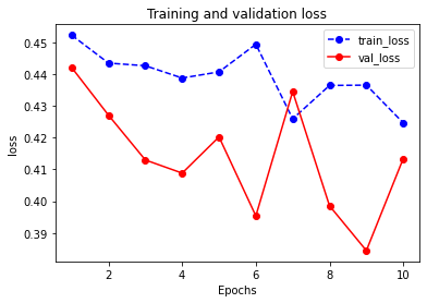
我们首先评估一下模型在训练集和验证集上的效果。
1 | dfhistory |
Results:
| epoch | loss | accuracy | val_loss | val_accuracy | |
|---|---|---|---|---|---|
| 0 | 1.0 | 0.452268 | 0.803371 | 0.442081 | 0.782609 |
| 1 | 2.0 | 0.443471 | 0.790730 | 0.427079 | 0.809783 |
| 2 | 3.0 | 0.442639 | 0.806180 | 0.412987 | 0.793478 |
| 3 | 4.0 | 0.438777 | 0.807584 | 0.408850 | 0.809783 |
| 4 | 5.0 | 0.440705 | 0.803371 | 0.420241 | 0.798913 |
| 5 | 6.0 | 0.449405 | 0.799157 | 0.395391 | 0.804348 |
| 6 | 7.0 | 0.425921 | 0.801966 | 0.434522 | 0.782609 |
| 7 | 8.0 | 0.436438 | 0.800562 | 0.398559 | 0.782609 |
| 8 | 9.0 | 0.436541 | 0.797753 | 0.384473 | 0.809783 |
| 9 | 10.0 | 0.424680 | 0.807584 | 0.413394 | 0.809783 |
Visualization
1
2
3
4
5
6
7
8
9
10
11
12
13
14
15import matplotlib.pyplot as plt
def plot_metric(dfhistory, metric):
train_metrics = dfhistory[metric]
val_metrics = dfhistory['val_'+metric]
epochs = range(1, len(train_metrics) + 1)
plt.plot(epochs, train_metrics, 'bo--')
plt.plot(epochs, val_metrics, 'ro-')
plt.title('Training and validation '+ metric)
plt.xlabel("Epochs")
plt.ylabel(metric)
plt.legend(["train_"+metric, 'val_'+metric])
plt.show()
plot_metric(dfhistory,"loss")Results:
1
plot_metric(dfhistory,"accuracy")
Results:

2.3.4 Predict
Probability
1
2y_pred_probs = net(torch.tensor(x_test[0:10]).float()).data
y_pred_probsResults:
1
2
3
4
5
6
7
8
9
10tensor([[0.0503],
[0.6572],
[0.3338],
[0.8437],
[0.5118],
[0.9191],
[0.1300],
[0.9312],
[0.5218],
[0.2221]])Classification
1
2
3y_pred = torch.where(y_pred_probs>0.5,
torch.ones_like(y_pred_probs),torch.zeros_like(y_pred_probs))
y_predResults:
1
2
3
4
5
6
7
8
9
10tensor([[0.],
[1.],
[0.],
[1.],
[1.],
[1.],
[0.],
[1.],
[1.],
[0.]])
2.3.5 Save model
Pytorch 有两种保存模型的方式,都是通过调用
pickle 序列化方法实现的。
- 只保存模型参数;
- 保存完整模型。
推荐使用第一种,第二种方法可能在切换设备和目录的时候出现各种问题。
1 | print(net.state_dict().keys()) |
Results:
1 | odict_keys(['linear1.weight', 'linear1.bias', 'linear2.weight', 'linear2.bias', 'linear3.weight', 'linear3.bias']) |
保存模型参数(\star\star\star)
1
2
3
4
5
6
7# 保存模型参数
torch.save(net.state_dict(), data_dir + "net_parameter.pkl")
net_clone = create_net()
net_clone.load_state_dict(torch.load(data_dir + "net_parameter.pkl"))
net_clone.forward(torch.tensor(x_test[0:10]).float()).dataResults:
1
2
3
4
5
6
7
8
9
10tensor([[0.0503],
[0.6572],
[0.3338],
[0.8437],
[0.5118],
[0.9191],
[0.1300],
[0.9312],
[0.5218],
[0.2221]])保存完整模型
1
2
3torch.save(net, data_dir + 'net_model.pkl')
net_loaded = torch.load(data_dir + 'net_model.pkl')
net_loaded(torch.tensor(x_test[0:10]).float()).dataResults:
1
2
3
4
5
6
7
8
9
10tensor([[0.0503],
[0.6572],
[0.3338],
[0.8437],
[0.5118],
[0.9191],
[0.1300],
[0.9312],
[0.5218],
[0.2221]])
3. Image classification
3.1 Data
3.1.1 Prepare data
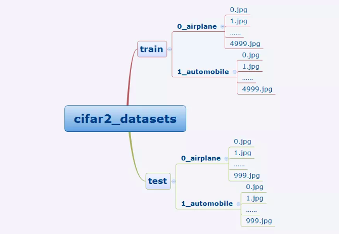
cifar2 数据集为 cifar10
数据集的子集,只包括前两种类别 airplane 和
automobile。
训练集有 airplane 和 automobile 图片各
5000 张,测试集有 airplane 和
automobile 图片各 1000 张。
cifar2 任务的目标是训练一个模型来对飞机
airplane 和机动车 automobile
两种图片进行分类。
我们准备的 Cifar2 数据集的文件结构如下所示。
在 Pytorch 中构建图片数据管道通常有两种方法。
使用
torchvision中的datasets.ImageFolder来读取图片然后用DataLoader来并行加载。通过继承
torch.utils.data.Dataset实现用户自定义读取逻辑然后用DataLoader来并行加载。
第二种方法是读取用户自定义数据集的通用方法,既可以读取图片数据集,也可以读取文本数据集。
本篇我们介绍第一种方法。
1 | import torch |
1 | def trasform_target(t): |
Results:
{'0_airplane': 0, '1_automobile': 1}Note: 原始的代码中,target_transform
使用了匿名函数
lambda:target_transform= lambda t:torch.tensor([t]).float(),虽然在此处不会报错,但在后面的迭代过程中会报
PicklingError 错误,错误信息如下:
1 | PicklingError: Can't pickle <function <lambda> at 0x000001D42D136310>: attribute lookup <lambda> on __main__ failed |
为了解决该问题,此处选择将该参数去掉,并手动对后面的
feature 和 labels 进行处理:
1 | features = features.float() |
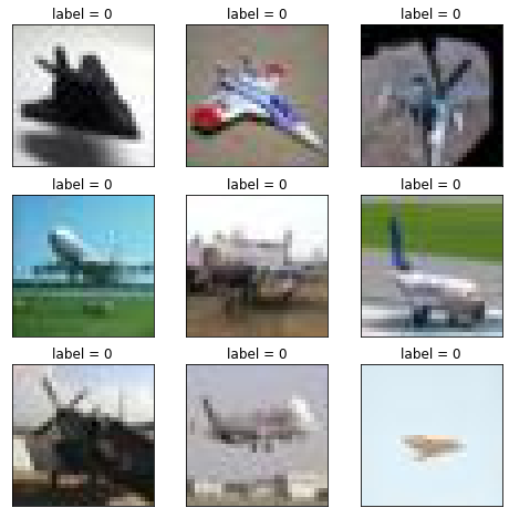
1 | #查看部分样本 |
Results:
Pytorch 的图片默认顺序是 Batch,
Channel, Width, Height
1 | # Pytorch的图片默认顺序是 Batch,Channel,Width,Height |
Results:
torch.Size([50, 3, 32, 32]) torch.Size([50])3.2 Model
3.2.1 Define model
上一章提到 Pytroch
通常有三种方式构建模型,此处选择通过继承 nn.Module
基类构建自定义模型。
1 | #测试AdaptiveMaxPool2d的效果 |
Results:
torch.Size([10, 8, 1, 1])1 | class Net(nn.Module): |
Results:
Net(
(conv1): Conv2d(3, 32, kernel_size=(3, 3), stride=(1, 1))
(pool): MaxPool2d(kernel_size=2, stride=2, padding=0, dilation=1, ceil_mode=False)
(conv2): Conv2d(32, 64, kernel_size=(5, 5), stride=(1, 1))
(dropout): Dropout2d(p=0.1, inplace=False)
(adaptive_pool): AdaptiveMaxPool2d(output_size=(1, 1))
(flatten): Flatten(start_dim=1, end_dim=-1)
(linear1): Linear(in_features=64, out_features=32, bias=True)
(relu): ReLU()
(linear2): Linear(in_features=32, out_features=1, bias=True)
(sigmoid): Sigmoid()
)产看模型概述
1
2import torchkeras
torchkeras.summary(net,input_shape= (3,32,32))Results:
1
2
3
4
5
6
7
8
9
10
11
12
13
14
15
16
17
18
19
20
21
22
23
24----------------------------------------------------------------
Layer (type) Output Shape Param #
================================================================
Conv2d-1 [-1, 32, 30, 30] 896
MaxPool2d-2 [-1, 32, 15, 15] 0
Conv2d-3 [-1, 64, 11, 11] 51,264
MaxPool2d-4 [-1, 64, 5, 5] 0
Dropout2d-5 [-1, 64, 5, 5] 0
AdaptiveMaxPool2d-6 [-1, 64, 1, 1] 0
Flatten-7 [-1, 64] 0
Linear-8 [-1, 32] 2,080
ReLU-9 [-1, 32] 0
Linear-10 [-1, 1] 33
Sigmoid-11 [-1, 1] 0
================================================================
Total params: 54,273
Trainable params: 54,273
Non-trainable params: 0
----------------------------------------------------------------
Input size (MB): 0.011719
Forward/backward pass size (MB): 0.359634
Params size (MB): 0.207035
Estimated Total Size (MB): 0.578388
----------------------------------------------------------------
3.2.2 Train model
Pytorch
通常需要用户编写自定义训练循环,训练循环的代码风格因人而异。
同样地,有 3 类典型的训练循环代码风格:
- 脚本形式训练循环;
- 函数形式训练循环;
- 类形式训练循环。
此处介绍一种较通用的函数形式训练循环。
1 | import pandas as pd |
定义训练循环的函数
1
len(dl_train)
Results:
2001
2
3
4
5
6
7
8
9
10
11
12
13
14
15
16
17
18
19
20
21
22
23
24
25
26
27
28
29
30
31
32
33
34
35
36
37
38def train_step(model,features,labels):
# 训练模式,dropout层发生作用
model.train()
# 梯度清零
model.optimizer.zero_grad()
# 正向传播求损失
predictions = model(features)
loss = model.loss_func(predictions,labels)
metric = model.metric_func(predictions,labels)
# 反向传播求梯度
loss.backward()
model.optimizer.step()
return loss.item(),metric.item()
def valid_step(model,features,labels):
# 预测模式,dropout层不发生作用
model.eval()
# 关闭梯度计算
with torch.no_grad():
predictions = model(features)
loss = model.loss_func(predictions,labels)
metric = model.metric_func(predictions,labels)
return loss.item(), metric.item()
# 测试train_step效果
features,labels = next(iter(dl_train))
# 手动对 features 和 labels 进行处理
features = features.float()
labels = labels.float().view(-1, 1)
train_step(model,features,labels)Results:
1
(0.7002284526824951, 0.6288998357963875)
Training
1
2
3
4
5
6
7
8
9
10
11
12
13
14
15
16
17
18
19
20
21
22
23
24
25
26
27
28
29
30
31
32
33
34
35
36
37
38
39
40
41
42
43
44
45
46
47
48
49
50
51
52
53
54
55
56
57
58
59def train_model(model,epochs,dl_train,dl_valid,log_step_freq):
metric_name = model.metric_name
dfhistory = pd.DataFrame(columns = ["epoch","loss",metric_name,"val_loss","val_"+metric_name])
print("Start Training...")
nowtime = datetime.datetime.now().strftime('%Y-%m-%d %H:%M:%S')
print("=========="*8 + "%s"%nowtime)
for epoch in range(1,epochs+1):
# 1,训练循环-------------------------------------------------
loss_sum = 0.0
metric_sum = 0.0
step = 1
for step, (features,labels) in enumerate(dl_train, 1):
features = features.float()
labels = labels.float().view(-1, 1)
loss,metric = train_step(model,features,labels)
# 打印batch级别日志
loss_sum += loss
metric_sum += metric
if step%log_step_freq == 0:
print(("[step = %d] loss: %.3f, "+metric_name+": %.3f") %
(step, loss_sum/step, metric_sum/step))
# 2,验证循环-------------------------------------------------
val_loss_sum = 0.0
val_metric_sum = 0.0
val_step = 1
for val_step, (features,labels) in enumerate(dl_valid, 1):
features = features.float()
labels = labels.float().view(-1, 1)
val_loss,val_metric = valid_step(model,features,labels)
val_loss_sum += val_loss
val_metric_sum += val_metric
# 3,记录日志-------------------------------------------------
info = (epoch, loss_sum/step, metric_sum/step,
val_loss_sum/val_step, val_metric_sum/val_step)
dfhistory.loc[epoch-1] = info
# 打印epoch级别日志
print(("\nEPOCH = %d, loss = %.3f,"+ metric_name + \
" = %.3f, val_loss = %.3f, "+"val_"+ metric_name+" = %.3f")
%info)
nowtime = datetime.datetime.now().strftime('%Y-%m-%d %H:%M:%S')
print("\n"+"=========="*8 + "%s"%nowtime)
print('Finished Training...')
return dfhistory
import datetime
epochs = 20
dfhistory = train_model(model,epochs,dl_train,dl_valid,log_step_freq = 50)Results:
1
2
3
4
5
6
7
8
9
10
11
12
13
14
15Start Training...
================================================================================2022-02-06 15:29:25
[step = 50] loss: 0.689, auc: 0.684
[step = 100] loss: 0.687, auc: 0.702
[step = 150] loss: 0.685, auc: 0.719
[step = 200] loss: 0.682, auc: 0.731
EPOCH = 1, loss = 0.682,auc = 0.731, val_loss = 0.669, val_auc = 0.798
...
EPOCH = 20, loss = 0.392,auc = 0.919, val_loss = 0.430, val_auc = 0.936
================================================================================2022-02-06 15:44:33
Finished Training...
3.2.3 Evaluate model
1 | dfhistory |
Results:
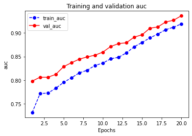
| epoch | loss | auc | val_loss | val_auc | |
|---|---|---|---|---|---|
| 0 | 1.0 | 0.681958 | 0.731338 | 0.668862 | 0.797954 |
| 1 | 2.0 | 0.654892 | 0.771506 | 0.627371 | 0.806149 |
| 2 | 3.0 | 0.608822 | 0.772492 | 0.569101 | 0.806107 |
| 3 | 4.0 | 0.569133 | 0.782751 | 0.537821 | 0.812113 |
| 4 | 5.0 | 0.547803 | 0.795203 | 0.516346 | 0.828602 |
| 5 | 6.0 | 0.535204 | 0.804953 | 0.501350 | 0.836900 |
| 6 | 7.0 | 0.524705 | 0.815323 | 0.501829 | 0.844522 |
| 7 | 8.0 | 0.516900 | 0.820933 | 0.484164 | 0.849198 |
| 8 | 9.0 | 0.507156 | 0.831129 | 0.473935 | 0.852870 |
| 9 | 10.0 | 0.501035 | 0.836087 | 0.494572 | 0.859365 |
| 10 | 11.0 | 0.490484 | 0.845260 | 0.458230 | 0.871329 |
| 11 | 12.0 | 0.481249 | 0.848306 | 0.447633 | 0.877395 |
| 12 | 13.0 | 0.470961 | 0.857883 | 0.467264 | 0.879283 |
| 13 | 14.0 | 0.458891 | 0.870709 | 0.420090 | 0.891266 |
| 14 | 15.0 | 0.447952 | 0.879920 | 0.426877 | 0.896159 |
| 15 | 16.0 | 0.439210 | 0.889682 | 0.392666 | 0.910185 |
| 16 | 17.0 | 0.424930 | 0.897675 | 0.459186 | 0.912733 |
| 17 | 18.0 | 0.416532 | 0.906937 | 0.426213 | 0.923270 |
| 18 | 19.0 | 0.406580 | 0.912283 | 0.377994 | 0.926940 |
| 19 | 20.0 | 0.392066 | 0.919133 | 0.429610 | 0.936487 |
1 | import matplotlib.pyplot as plt |
Results:
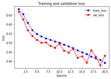
1 | plot_metric(dfhistory,"auc") |
Results:
3.2.4 Predict
1 | def predict(model,dl): |
Probability
1
2y_pred_probs = predict(model,dl_valid)
y_pred_probsResults:
1
2
3
4
5
6
7tensor([[0.9675],
[0.6920],
[0.1920],
...,
[0.9491],
[0.8573],
[0.9429]])Classification
1
torch.ones_like(y_pred_probs),torch.zeros_like(y_pred_probs)
Results:
1
2
3
4
5
6
7
8
9
10
11
12
13
14(tensor([[1.],
[1.],
[1.],
...,
[1.],
[1.],
[1.]]),
tensor([[0.],
[0.],
[0.],
...,
[0.],
[0.],
[0.]]))
3.2.5 Save model
1 | print(model.state_dict().keys()) |
Results:
odict_keys(['conv1.weight', 'conv1.bias', 'conv2.weight', 'conv2.bias',
'linear1.weight', 'linear1.bias', 'linear2.weight', 'linear2.bias'])Save parameters
1
2
3
4
5
6
7
8# 保存模型参数
torch.save(model.state_dict(), data_dir + "model_parameter.pkl")
net_clone = Net()
net_clone.load_state_dict(torch.load(data_dir + "model_parameter.pkl"))
predict(net_clone,dl_valid)Results:
1
2
3
4
5
6
7tensor([[0.6056],
[0.9186],
[0.9777],
...,
[0.9546],
[0.2568],
[0.9221]])
4. Text classification
4.1 Data
4.1.1 Prepare data
imdb
数据集的目标是根据电影评论的文本内容预测评论的情感标签。
训练集有 20000
条电影评论文本,测试集有5000条电影评论文本,其中正面评论和负面评论都各占一半。
文本数据预处理较为繁琐,包括中文切词(本示例不涉及),构建词典,编码转换,序列填充,构建数据管道等等。
在 torch 中预处理文本数据一般使用 torchtext
或者自定义 Dataset,torchtext
功能非常强大,可以构建文本分类,序列标注,问答模型,机器翻译等
NLP 任务的数据集。
下面仅演示使用它来构建文本分类数据集的方法。
较完整的教程可以参考以下知乎文章:《pytorch学习笔记—Torchtext》
torchtext常见API一览torchtext.data.Example: 用来表示一个样本,数据和标签torchtext.vocab.Vocab: 词汇表,可以导入一些预训练词向量torchtext.data.Datasets: 数据集类,__getitem__返回Example实例,torchtext.data.TabularDataset是其子类。torchtext.data.Field: 用来定义字段的处理方法(文本字段,标签字段)创建Example时的 预处理,batch 时的一些处理操作。torchtext.data.Iterator: 迭代器,用来生成batchtorchtext.datasets: 包含了常见的数据集。
1 | import torch |
Note:TabularDataset 和
Field 在新版的 TorchText 中不再位于
torchtext.data,而是在 torchtext.legacy.data
中。
查看
example信息1
2
3#查看example信息
print(ds_train[0].text)
print(ds_train[0].label)Results:
1
2
3
4
5
6
7
8
9
10
11
12
13
14
15
16
17
18
19
20
21
22
23
24
25
26
27
28
29
30
31
32
33
34
35['it', 'really', 'boggles', 'my', 'mind', 'when', 'someone', 'comes',
'across', 'a', 'movie', 'like', 'this', 'and', 'claims', 'it', 'to',
'be', 'one', 'of', 'the', 'worst', 'slasher', 'films', 'out', 'there',
'this', 'is', 'by', 'far', 'not', 'one', 'of', 'the', 'worst', 'out',
'there', 'still', 'not', 'a', 'good', 'movie', 'but', 'not', 'the',
'worst', 'nonetheless', 'go', 'see', 'something', 'like', 'death',
'nurse', 'or', 'blood', 'lake', 'and', 'then', 'come', 'back', 'to',
'me', 'and', 'tell', 'me', 'if', 'you', 'think', 'the', 'night',
'brings', 'charlie', 'is', 'the', 'worst', 'the', 'film', 'has',
'decent', 'camera', 'work', 'and', 'editing', 'which', 'is', 'way',
'more', 'than', 'i', 'can', 'say', 'for', 'many', 'more', 'extremely',
'obscure', 'slasher', 'filmsbr', 'br', 'the', 'film', 'doesnt',
'deliver', 'on', 'the', 'onscreen', 'deaths', 'theres', 'one', 'death',
'where', 'you', 'see', 'his', 'pruning', 'saw', 'rip', 'into', 'a',
'neck', 'but', 'all', 'other', 'deaths', 'are', 'hardly', 'interesting',
'but', 'the', 'lack', 'of', 'onscreen', 'graphic', 'violence', 'doesnt',
'mean', 'this', 'isnt', 'a', 'slasher', 'film', 'just', 'a', 'bad',
'onebr', 'br', 'the', 'film', 'was', 'obviously', 'intended', 'not',
'to', 'be', 'taken', 'too', 'seriously', 'the', 'film', 'came', 'in',
'at', 'the', 'end', 'of', 'the', 'second', 'slasher', 'cycle', 'so',
'it', 'certainly', 'was', 'a', 'reflection', 'on', 'traditional',
'slasher', 'elements', 'done', 'in', 'a', 'tongue', 'in', 'cheek', 'way',
'for', 'example', 'after', 'a', 'kill', 'charlie', 'goes', 'to', 'the',
'towns', 'welcome', 'sign', 'and', 'marks', 'the', 'population', 'down',
'one', 'less', 'this', 'is', 'something', 'that', 'can', 'only', 'get',
'a', 'laughbr', 'br', 'if', 'youre', 'into', 'slasher', 'films',
'definitely', 'give', 'this', 'film', 'a', 'watch', 'it', 'is',
'slightly', 'different', 'than', 'your', 'usual', 'slasher', 'film',
'with', 'possibility', 'of', 'two', 'killers', 'but', 'not', 'by',
'much', 'the', 'comedy', 'of', 'the', 'movie', 'is', 'pretty', 'much',
'telling', 'the', 'audience', 'to', 'relax', 'and', 'not', 'take', 'the',
'movie', 'so', 'god', 'darn', 'serious', 'you', 'may', 'forget', 'the',
'movie', 'you', 'may', 'remember', 'it', 'ill', 'remember', 'it',
'because', 'i', 'love', 'the', 'name']
0查看词典信息
1
print(len(TEXT.vocab))
Results:
1
108197
itos: index to string
1
2
3# itos: index to string
print(TEXT.vocab.itos[0])
print(TEXT.vocab.itos[1])Results:
1
2<unk>
<pad>stoi: string to index
1
2
3# stoi: string to index
print(TEXT.vocab.stoi['<unk>']) #unknown 未知词
print(TEXT.vocab.stoi['<pad>']) #padding 填充Results:
1
20
1词频
1
2
3
4# freqs: 词频
print(TEXT.vocab.freqs['<unk>'])
print(TEXT.vocab.freqs['a'])
print(TEXT.vocab.freqs['good'])Results:
1
2
30
129453
11457查看数据管道信息
1
2
3
4
5
6
7
8
9# 查看数据管道信息
# 注意有坑:text第0维是句子长度
for batch in train_iter:
features = batch.text
labels = batch.label
print(features)
print(features.shape)
print(labels)
breakResults:
1
2
3
4
5
6
7
8
9tensor([[ 9, 11, 9, ..., 10, 2, 10],
[ 921, 7, 7, ..., 628, 902, 283],
[ 15, 29, 1651, ..., 6, 172, 11],
...,
[ 7, 522, 461, ..., 1, 1, 1],
[ 205, 8, 108, ..., 1, 1, 1],
[ 0, 11, 4, ..., 1, 1, 1]])
torch.Size([200, 20])
tensor([1, 1, 1, 0, 1, 0, 0, 1, 0, 0, 1, 0, 0, 0, 1, 1, 0, 1, 0, 1])
4.1.2 数据管道转换
将数据管道组织成 torch.utils.data.DataLoader 相似的
features, label 输出形式。
1 | # 将数据管道组织成torch.utils.data.DataLoader相似的features,label输出形式 |
4.2 Model
4.2.1 Define model
第二章提到使用 Pytorch
通常有三种方式构建模型,此处选择使用第三种方式进行构建。
1 | import torch |
Results:
Net(
(embedding): Embedding(10000, 3, padding_idx=1)
(conv): Sequential(
(conv_1): Conv1d(3, 16, kernel_size=(5,), stride=(1,))
(pool_1): MaxPool1d(kernel_size=2, stride=2, padding=0, dilation=1, ceil_mode=False)
(relu_1): ReLU()
(conv_2): Conv1d(16, 128, kernel_size=(2,), stride=(1,))
(pool_2): MaxPool1d(kernel_size=2, stride=2, padding=0, dilation=1, ceil_mode=False)
(relu_2): ReLU()
)
(dense): Sequential(
(flatten): Flatten(start_dim=1, end_dim=-1)
(linear): Linear(in_features=6144, out_features=1, bias=True)
(sigmoid): Sigmoid()
)
)
----------------------------------------------------------------
Layer (type) Output Shape Param #
================================================================
Embedding-1 [-1, 200, 3] 30,000
Conv1d-2 [-1, 16, 196] 256
MaxPool1d-3 [-1, 16, 98] 0
ReLU-4 [-1, 16, 98] 0
Conv1d-5 [-1, 128, 97] 4,224
MaxPool1d-6 [-1, 128, 48] 0
ReLU-7 [-1, 128, 48] 0
Flatten-8 [-1, 6144] 0
Linear-9 [-1, 1] 6,145
Sigmoid-10 [-1, 1] 0
================================================================
Total params: 40,625
Trainable params: 40,625
Non-trainable params: 0
----------------------------------------------------------------
Input size (MB): 0.000763
Forward/backward pass size (MB): 0.287796
Params size (MB): 0.154972
Estimated Total Size (MB): 0.443531
----------------------------------------------------------------4.2.2 Training model
训练 Pytorch
通常需要用户编写自定义训练循环,训练循环的代码风格因人而异。
有 3
类典型的训练循环代码风格:脚本形式训练循环,函数形式训练循环,类形式训练循环。
此处介绍一种类形式的训练循环。
我们利用 Pytorch-Lightning 定义了一个高阶的模型接口
LightModel, 封装在 torchkeras 中,
可以非常方便地训练模型。
1 | import pytorch_lightning as pl |
Note:第六行中原始的 metrics 为
pl.metrics,但最新的版本中 metrics
已经被移到新的包torchmetrics 。
1 | pl.seed_everything(1234) |
Results:
1 | Global seed set to 1234 |
4.2.3 Evaluate model
1 | import pandas as pd |
Results:
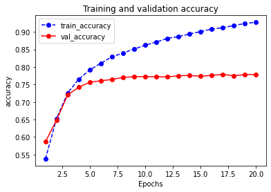
| val_loss | val_accuracy | loss | accuracy | epoch | |
|---|---|---|---|---|---|
| 0 | 0.668126 | 0.5870 | 0.694043 | 0.538100 | 0 |
| 1 | 0.622295 | 0.6486 | 0.619329 | 0.653051 | 1 |
| 2 | 0.543876 | 0.7202 | 0.539137 | 0.725501 | 2 |
| 3 | 0.516527 | 0.7420 | 0.485453 | 0.765250 | 3 |
| 4 | 0.501172 | 0.7566 | 0.446320 | 0.791349 | 4 |
| 5 | 0.493917 | 0.7606 | 0.416267 | 0.810600 | 5 |
| 6 | 0.491973 | 0.7642 | 0.390249 | 0.828950 | 6 |
| 7 | 0.485185 | 0.7702 | 0.367199 | 0.839549 | 7 |
| 8 | 0.486927 | 0.7722 | 0.348247 | 0.851001 | 8 |
| 9 | 0.487843 | 0.7724 | 0.329982 | 0.862001 | 9 |
| 10 | 0.490562 | 0.7718 | 0.312720 | 0.870900 | 10 |
| 11 | 0.506245 | 0.7718 | 0.297354 | 0.881451 | 11 |
| 12 | 0.498210 | 0.7748 | 0.283493 | 0.886551 | 12 |
| 13 | 0.501044 | 0.7758 | 0.270271 | 0.893802 | 13 |
| 14 | 0.519616 | 0.7736 | 0.257364 | 0.901002 | 14 |
| 15 | 0.517258 | 0.7760 | 0.245659 | 0.907853 | 15 |
| 16 | 0.522427 | 0.7788 | 0.234360 | 0.911853 | 16 |
| 17 | 0.525286 | 0.7750 | 0.223529 | 0.918153 | 17 |
| 18 | 0.533164 | 0.7780 | 0.213193 | 0.923954 | 18 |
| 19 | 0.540092 | 0.7786 | 0.204244 | 0.927404 | 19 |
Visualization
1
2
3
4
5
6
7
8
9
10
11
12
13
14
15import matplotlib.pyplot as plt
def plot_metric(dfhistory, metric):
train_metrics = dfhistory[metric]
val_metrics = dfhistory['val_'+metric]
epochs = range(1, len(train_metrics) + 1)
plt.plot(epochs, train_metrics, 'bo--')
plt.plot(epochs, val_metrics, 'ro-')
plt.title('Training and validation '+ metric)
plt.xlabel("Epochs")
plt.ylabel(metric)
plt.legend(["train_"+metric, 'val_'+metric])
plt.show()
plot_metric(dfhistory,"loss")Results:

1
plot_metric(dfhistory,"accuracy")
Results:
Evaluate
1
2
3# 评估
results = trainer.test(model, test_dataloaders=dl_valid, verbose = False)
print(results[0])Results:
1
2
3Testing: 0it [00:00, ?it/s]
{'test_loss': 0.5400923490524292, 'test_accuracy': 0.7785999774932861}
4.2.4 Predict
1 | def predict(model,dl): |
Results:
tensor([[0.0053],
[0.9006],
[0.1638],
...,
[0.9836],
[0.5532],
[0.0018]])4.2.5 Save model
1 | print(ckpt_cb.best_model_score) |
Results:
1 | tensor(0.4852) |
5. Time series regression
5.1 Introduction
2020年
发生的新冠肺炎疫情灾难给各国人民的生活造成了诸多方面的影响。
有的同学是收入上的,有的同学是感情上的,有的同学是心理上的,还有的同学是体重上的。
本文基于中国 2020 年 3
月之前的疫情数据,建立时间序列 RNN
模型,对中国的新冠肺炎疫情结束时间进行预测。
5.2 Data
5.2.1 Prepare data
本文的数据集取自tushare,获取该数据集的方法参考了以下文章。
《https://zhuanlan.zhihu.com/p/109556102》
1 | data_dir = '../data/' |
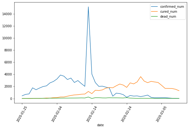
总数
1
2
3
4
5
6
7import numpy as np
import pandas as pd
import matplotlib.pyplot as plt
df = pd.read_csv(data_dir + "covid-19.csv",sep = "\t")
df.plot(x = "date",y = ["confirmed_num","cured_num","dead_num"],figsize=(10,6))
plt.xticks(rotation=60);Results:

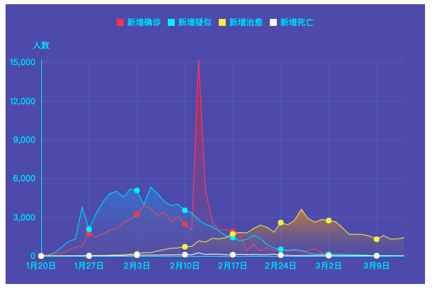
新增
1
2
3
4
5
6
7dfdata = df.set_index("date")
dfdiff = dfdata.diff(periods=1).dropna()
dfdiff = dfdiff.reset_index("date")
dfdiff.plot(x = "date",y = ["confirmed_num","cured_num","dead_num"],figsize=(10,6))
plt.xticks(rotation=60)
dfdiff = dfdiff.drop("date",axis = 1).astype("float32")Results:
1
dfdiff.head()
Results:
confirmed_num
cured_num
dead_num
0
457.0
4.0
16.0
1
688.0
11.0
15.0
2
769.0
2.0
24.0
3
1771.0
9.0
26.0
4
1459.0
43.0
26.0
5.2.2 Dataloader
下面我们通过继承 torch.utils.data.Dataset
实现自定义时间序列数据集。
torch.utils.data.Dataset
是一个抽象类,用户想要加载自定义的数据只需要继承这个类,并且覆写其中的两个方法即可:
__len__:实现len(dataset)返回整个数据集的大小。__getitem__:用来获取一些索引的数据,使dataset[i]返回数据集中第i个样本。
不覆写这两个方法会直接返回错误。
1 | import torch |
5.3 Model
5.3.1 Define model
前面提到使用 Pytorch 通常有三种方式构建模型:
- 使用
nn.Sequential按层顺序构建模型; - 继承
nn.Module基类构建自定义模型; - 继承nn.Module基类构建模型并辅助应用模型容器进行封装。
此处选择第二种方式构建模型。
由于接下来使用类形式的训练循环,我们进一步将模型封装成
torchkeras 中的 Model 类来获得类似
Keras 中高阶模型接口的功能。Model
类实际上继承自 nn.Module 类。
1 | import torch |
Results:
Model(
  (net): Net(
    (lstm): LSTM(3, 3, num_layers=5, batch_first=True)
    (linear): Linear(in_features=3, out_features=3, bias=True)
    (block): Block()
  )
)
----------------------------------------------------------------
        Layer (type)               Output Shape         Param #
================================================================
              LSTM-1                 [-1, 8, 3]             480
            Linear-2                    [-1, 3]              12
             Block-3                    [-1, 3]               0
================================================================
Total params: 492
Trainable params: 492
Non-trainable params: 0
----------------------------------------------------------------
Input size (MB): 0.000092
Forward/backward pass size (MB): 0.000229
Params size (MB): 0.001877
Estimated Total Size (MB): 0.002197
----------------------------------------------------------------
5.3.2 Training model
训练 Pytorch
通常需要用户编写自定义训练循环,训练循环的代码风格因人而异。
有 3 类典型的训练循环代码风格:
- 脚本形式训练循环;
- 函数形式训练循环;
- 类形式训练循环。
此处介绍一种类形式的训练循环。
我们仿照 Keras 定义了一个高阶的模型接口
Model, 实现 fit,
validate,predict, summary
方法,相当于用户自定义高阶API。
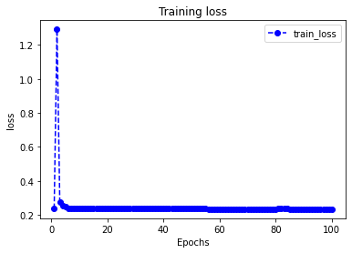
注:循环神经网络调试较为困难,需要设置多个不同的学习率多次尝试,以取得较好的效果。
1 | def mspe(y_pred,y_true): |
Resulst:
1 | Start Training ... |
5.3.3 Evaluate model
评估模型一般要设置验证集或者测试集,由于此例数据较少,我们仅仅可视化损失函数在训练集上的迭代情况。
1 | import matplotlib.pyplot as plt |
Results:
5.3.4 Predict
此处我们使用模型预测疫情结束时间,即新增确诊病例为 0
的时间。
使用
dfresult记录现有数据以及此后预测的疫情数据1
2
3#使用dfresult记录现有数据以及此后预测的疫情数据
dfresult = dfdiff[["confirmed_num","cured_num","dead_num"]].copy()
dfresult.tail()Results:
confirmed_num
cured_num
dead_num
41
143.0
1681.0
30.0
42
99.0
1678.0
28.0
43
44.0
1661.0
27.0
44
40.0
1535.0
22.0
45
19.0
1297.0
17.0
预测此后
200天的新增走势,将其结果添加到dfresult中1
2
3
4
5
6
7
8#预测此后200天的新增走势,将其结果添加到dfresult中
for i in range(200):
arr_input = torch.unsqueeze(torch.from_numpy(dfresult.values[-38:,:]),axis=0)
arr_predict = model.forward(arr_input)
dfpredict = pd.DataFrame(torch.floor(arr_predict).data.numpy(),
columns = dfresult.columns)
dfresult = dfresult.append(dfpredict,ignore_index=True)查询新增确诊为零的日期
1
dfresult.query("confirmed_num==0").head()
Results:
confirmed_num
cured_num
dead_num
50
0.0
1006.0
3.0
51
0.0
956.0
2.0
52
0.0
909.0
1.0
53
0.0
864.0
0.0
54
0.0
821.0
0.0
第 50 天开始新增确诊降为 0,第
45 天对应 3 月 10 日,也就是
5 天后,即预计 3 月 15
日新增确诊降为 0。
注:该预测偏乐观。
新增治愈人数为零
1
dfresult.query("cured_num==0").head()
Results:
confirmed_num
cured_num
dead_num
140
0.0
0.0
0.0
141
0.0
0.0
0.0
142
0.0
0.0
0.0
143
0.0
0.0
0.0
144
0.0
0.0
0.0
第 132 天开始新增治愈降为 0,第
45 天对应 3 月 10 日,也就是大概
3 个月后,即 6 月 10
日左右全部治愈。
注: 该预测偏悲观,并且存在问题,如果将每天新增治愈人数加起来,将超过累计确诊人数。
5.3.5 Save model
推荐使用保存参数方式保存模型。
1 | # 保存模型参数 |
Results:
{'val_loss': 0.23351764678955078}