1. Introduction
1.1 Preface
本系列博文是和鲸社区的活动《20天吃掉那只PyTorch》学习的笔记,本篇为系列笔记的第二篇——
Pytorch 的核心概念。该专栏是 Github 上
2.8K
星的项目,在学习该书的过程中可以参考阅读《Python深度学习》一书的第一部分"深度学习基础"内容。
《Python深度学习》这本书是 Keras 之父
Francois Chollet
所著,该书假定读者无任何机器学习知识,以Keras
为工具,使用丰富的范例示范深度学习的最佳实践,该书通俗易懂,全书没有一个数学公式,注重培养读者的深度学习直觉。
《Python深度学习》一书的第一部分的 4
个章节内容如下,预计读者可以在 20 小时之内学完。
- 什么是深度学习
- 神经网络的数学基础
- 神经网络入门
- 机器学习基础
本系列博文的大纲如下:
- 一、PyTorch的建模流程
- 二、PyTorch的核心概念
- 三、PyTorch的层次结构
- 四、PyTorch的低阶API
- 五、PyTorch的中阶API
- 六、PyTorch的高阶API
最后,本博文提供所使用的全部数据,读者可以从下述连接中下载数据:
1.2 Pytorch 的核心概念
Pytorch
是一个基于Python的机器学习库。它广泛应用于计算机视觉,自然语言处理等深度学习领域。是目前和TensorFlow
分庭抗礼的深度学习框架,在学术圈颇受欢迎。
它主要提供了以下两种核心功能:
- 支持
GPU加速的张量计算。 - 方便优化模型的自动微分机制。
Pytorch的主要优点:
简洁易懂:
Pytorch的API设计的相当简洁一致。基本上就是tensor,autograd,nn三级封装。学习起来非常容易。有一个这样的段子,说三大框架的设计哲学如下:TensorFlow: Make it complicated
Keras: Make it complicated and hide it
Pytorch: Keep it simple and stupid.
便于调试:
Pytorch采用动态图,可以像普通Python代码一样进行调试。不同于TensorFlow,Pytorch的报错说明通常很容易看懂。有一个这样的段子,说你永远不可能从
TensorFlow的报错说明中找到它出错的原因。强大高效:
Pytorch提供了非常丰富的模型组件,可以快速实现想法。并且运行速度很快。目前大部分深度学习相关的Paper都是用Pytorch实现的。有些研究人员表示,从使用
TensorFlow转换为使用Pytorch之后,他们的睡眠好多了,头发比以前浓密了,皮肤也比以前光滑了。
俗话说,万丈高楼平地起,Pytorch
这座大厦也有它的地基。
Pytorch
底层最核心的概念是张量,动态计算图以及自动微分。
2. Tensor data structure
2.1 Tensor
张量的数据类型和 numpy.array 基本一一对应,但是不支持
str 类型。
包括:
- torch.float64(torch.double);
- torch.float32(torch.float);
- torch.float16;
- torch.int64(torch.long);
- torch.int32(torch.int);
- torch.int16;
- torch.int8;
- torch.uint8;
- torch.bool.
一般神经网络建模使用的都是 torch.float32 类型。
2.1.1 Data type
自动推断数据类型
1
2
3
4
5
6
7
8
9
10
import numpy as np
import torch
# 自动推断数据类型
i = torch.tensor(1)
print(i,i.dtype)
x = torch.tensor(2.0)
print(x,x.dtype)
b = torch.tensor(True)
print(b,b.dtype)Results:
1
2
3
tensor(1) torch.int64
tensor(2.) torch.float32
tensor(True) torch.bool指定数据类型
1
2
3
4
# 指定数据类型
i = torch.tensor(1,dtype = torch.int32);print(i,i.dtype)
x = torch.tensor(2.0,dtype = torch.double);print(x,x.dtype)Results:
  tensor(1, dtype=torch.int32) torch.int32
  tensor(2., dtype=torch.float64) torch.float64
使用特定类型构造函数
1
2
3
i = torch.IntTensor(1);print(i,i.dtype)
x = torch.Tensor(np.array(2.0));print(x,x.dtype) # 等价于torch.FloatTensor
b = torch.BoolTensor(np.array([1,0,2,0])); print(b,b.dtype)Results:
  tensor([1], dtype=torch.int32) torch.int32
  tensor(2.) torch.float32
  tensor([ True, False,  True, False]) torch.bool
不同类型进行转换
1
2
3
4
i = torch.tensor(1); print(i,i.dtype)
x = i.float(); print(x,x.dtype) #调用 float方法转换成浮点类型
y = i.type(torch.float); print(y,y.dtype) #使用type函数转换成浮点类型
z = i.type_as(x);print(z,z.dtype) #使用type_as方法转换成某个Tensor相同类型Results:
  tensor(1) torch.int64
  tensor(1.) torch.float32
  tensor(1.) torch.float32
  tensor(1.) torch.float32
2.2 Dimension of tensor
不同类型的数据可以用不同维度(dimension)的张量来表示。
- 标量:
0维张量; - 向量:
1维张量; - 矩阵:
2维张量。
彩色图像有 rgb 三个通道,可以表示为 3
维张量。视频还有时间维,可以表示为 4 维张量。
Note:可以简单地总结为:有几层中括号,就是多少维的张量。
Scalar
1
2
3
scalar = torch.tensor(True)
print(scalar)
print(scalar.dim()) # 标量,0维张量Results:
  tensor(True)
  0
Vector
1
2
3
vector = torch.tensor([1.0,2.0,3.0,4.0]) #向量,1维张量
print(vector)
print(vector.dim())Results:
  tensor([1., 2., 3., 4.])
  1
Matrix
1
2
3
tensor3 = torch.tensor([[[1.0,2.0],[3.0,4.0]],[[5.0,6.0],[7.0,8.0]]]) # 3维张量
print(tensor3)
print(tensor3.dim())Results:
1
2
3
4
5
6
tensor([[[1., 2.],
[3., 4.]],
[[5., 6.],
[7., 8.]]])
34-D tensor
1
2
3
4
tensor4 = torch.tensor([[[[1.0,1.0],[2.0,2.0]],[[3.0,3.0],[4.0,4.0]]],
[[[5.0,5.0],[6.0,6.0]],[[7.0,7.0],[8.0,8.0]]]]) # 4维张量
print(tensor4)
print(tensor4.dim())Results:
1
2
3
4
5
6
7
8
9
10
11
12
13
tensor([[[[1., 1.],
[2., 2.]],
[[3., 3.],
[4., 4.]]],
[[[5., 5.],
[6., 6.]],
[[7., 7.],
[8., 8.]]]])
4
2.3 Size of tensor
几个常用的跟大小相关的方法: - shape
可以使用 `shape` 属性或者 `size()` 方法查看张量在每一维的长度,view
可以使用
view方法改变张量的尺寸。reshape
如果
view方法改变尺寸失败,可以使用reshape方法.1
2
3vector = torch.tensor([1.0,2.0,3.0,4.0])
print(vector.size())
print(vector.shape)Results:
1
2
3
4
5
6
7
8
9
10
11
12
13
14
15
16
17
18
19torch.Size([4])
torch.Size([4])
- view 改变张量尺寸
```python
# 使用view可以改变张量尺寸
vector = torch.arange(0,12)
print(vector)
print(vector.shape)
matrix34 = vector.view(3,4)
print(matrix34)
print(matrix34.shape)
matrix43 = vector.view(4,-1) #-1表示该位置长度由程序自动推断
print(matrix43)
print(matrix43.shape)Results:
  tensor([ 0,  1,  2,  3,  4,  5,  6,  7,  8,  9, 10, 11])
  torch.Size([12])
  tensor([[ 0,  1,  2,  3],
          [ 4,  5,  6,  7],
          [ 8,  9, 10, 11]])
  torch.Size([3, 4])
  tensor([[ 0,  1,  2],
          [ 3,  4,  5],
          [ 6,  7,  8],
          [ 9, 10, 11]])
  torch.Size([4, 3])
reshape 方法
有些操作会让张量存储结构扭曲,直接使用
view会失败,可以用reshape方法1
2
3
4
5
6
7
8
9
10
11
12
13
14# 有些操作会让张量存储结构扭曲,直接使用view会失败,可以用reshape方法
matrix26 = torch.arange(0,12).view(2,6)
print(matrix26)
print(matrix26.shape)
# 转置操作让张量存储结构扭曲
matrix62 = matrix26.t()
print(matrix62.is_contiguous())
# 直接使用view方法会失败,可以使用reshape方法
#matrix34 = matrix62.view(3,4) #error!
matrix34 = matrix62.reshape(3,4) #等价于matrix34 = matrix62.contiguous().view(3,4)
print(matrix34)Results:
1
2
3
4
5
6
7tensor([[ 0, 1, 2, 3, 4, 5],
[ 6, 7, 8, 9, 10, 11]])
torch.Size([2, 6])
False
tensor([[ 0, 6, 1, 7],
[ 2, 8, 3, 9],
[ 4, 10, 5, 11]])
2.4 Tensor and numpy array
可以用 numpy 方法从 Tensor 得到
numpy 数组,也可以用 torch.from_numpy 从
numpy 数组得到 Tensor。
Note:这两种方法关联的 Tensor 和
numpy
数组是共享数据内存的。如果改变其中一个,另外一个的值也会发生改变。
如果有需要,可以: 1. 用张量的 clone
方法拷贝张量,中断这种关联。 2. 使用 item
方法从标量张量得到对应的 Python 数值。 3.
使用tolist方法从张量得到对应的Python数值列表。
from_numpy()1
2
3
4
5
6
7
8
9
10
11
12
13
14
15import numpy as np
import torch
#torch.from_numpy函数从numpy数组得到Tensor
arr = np.zeros(3)
tensor = torch.from_numpy(arr)
print("before add 1:")
print(arr)
print(tensor)
print("\nafter add 1:")
np.add(arr,1, out = arr) #给 arr增加1,tensor也随之改变
print(arr)
print(tensor)Results:
before add 1: [0. 0. 0.] tensor([0., 0., 0.], dtype=torch.float64) after add 1: [1. 1. 1.] tensor([1., 1., 1.], dtype=torch.float64)numpy()1
2
3
4
5
6
7
8
9
10
11
12
13
14
15# numpy方法从Tensor得到numpy数组
tensor = torch.zeros(3)
arr = tensor.numpy()
print("before add 1:")
print(tensor)
print(arr)
print("\nafter add 1:")
#使用带下划线的方法表示计算结果会返回给调用 张量
tensor.add_(1) #给 tensor增加1,arr也随之改变
#或: torch.add(tensor,1,out = tensor)
print(tensor)
print(arr)Results:
before add 1: tensor([0., 0., 0.]) [0. 0. 0.] after add 1: tensor([1., 1., 1.]) [1. 1. 1.]clone()可以用clone() 方法拷贝张量,中断这种关联
1
2
3
4
5
6
7
8
9
10
11
12
13
14tensor = torch.zeros(3)
#使用clone方法拷贝张量, 拷贝后的张量和原始张量内存独立
arr = tensor.clone().numpy() # 也可以使用tensor.data.numpy()
print("before add 1:")
print(tensor)
print(arr)
print("\nafter add 1:")
#使用 带下划线的方法表示计算结果会返回给调用 张量
tensor.add_(1) #给 tensor增加1,arr不再随之改变
print(tensor)
print(arr)Results:
before add 1: tensor([0., 0., 0.]) [0. 0. 0.] after add 1: tensor([1., 1., 1.]) [0. 0. 0.]tolist()1
2
3
4
5
6
7
8
9
10# item方法和tolist方法可以将张量转换成Python数值和数值列表
scalar = torch.tensor(1.0)
s = scalar.item()
print(s)
print(type(s))
tensor = torch.rand(2,2)
t = tensor.tolist()
print(t)
print(type(t))Results:
1.0 <class 'float'> [[0.6784629225730896, 0.811877429485321], [0.28022295236587524, 0.9736372828483582]] <class 'list'>
3. Auto differentiation mechanism
神经网络通常依赖反向传播求梯度来更新网络参数,求梯度过程通常是一件非常复杂而容易出错的事情。而深度学习框架可以帮助我们自动地完成这种求梯度运算。
Pytorch 一般通过反向传播 backward 方法
实现这种求梯度计算。该方法求得的梯度将存在对应自变量张量的
grad 属性下。除此之外,也能够调用
torch.autograd.grad 函数来实现求梯度计算。这就是
Pytorch 的自动微分机制。
3.1 利用 backward 方法求导数
backward
方法通常在一个标量张量上调用,该方法求得的梯度将存在对应自变量张量的
grad 属性下。如果调用的张量非标量,则要传入一个和它同形状的
gradient 参数张量。相当于用该 gradient
参数张量与调用张量作向量点乘,得到的标量结果再反向传播。
3.1.1 标量的反向传播
1 | import numpy as np |
Results:
tensor(-2.)3.1.2 非标量的反向传播
1 | import numpy as np |
Results:
x:
tensor([[0., 0.],
[1., 2.]], requires_grad=True)
y:
tensor([[1., 1.],
[0., 1.]], grad_fn=<AddBackward0>)
x_grad:
tensor([[-2., -2.],
[ 0., 2.]])3.1.3 非标量的反向传播可以用标量的反向传播实现
1 | import numpy as np |
Results:
x: tensor([[0., 0.],
[1., 2.]], requires_grad=True)
y: tensor([[1., 1.],
[0., 1.]], grad_fn=<AddBackward0>)
x_grad:
tensor([[-2., -2.],
[ 0., 2.]])3.2 利用autograd.grad方法求导数
3.2.1 单变量求导
1 | import numpy as np |
Results:
tensor(-2.)
tensor(2.)3.2.2 多变量求导
1 | import numpy as np |
Results:
tensor(2.) tensor(1.)
tensor(3.) tensor(2.)3.3 利用自动微分和优化器求最小值
1 | import numpy as np |
Results:
y= tensor(0.) ; x= tensor(1.0000)4. 动态计算图
本节学习 Pytorch 的动态计算图。
包括:
- 动态计算图简介
- 计算图中的Function
- 计算图和反向传播
- 叶子节点和非叶子节点
- 计算图在TensorBoard中的可视化
4.1 动态计算图简介
Pytorch 的计算图由节点和边组成,节点表示张量或者
Function,边表示张量和 Function
之间的依赖关系。
Pytorch
中的计算图是动态图。这里的动态主要有两重含义:
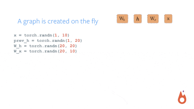
计算图的正向传播是立即执行的。无需等待完整的计算图创建完毕,每条语句都会在计算图中动态添加节点和边,并立即执行正向传播得到计算结果。
计算图在反向传播后立即销毁。下次调用需要重新构建计算图。如果在程序中使用了
backward方法执行了反向传播,或者利用torch.autograd.grad方法计算了梯度,那么创建的计算图会被立即销毁,释放存储空间,下次调用需要重新创建。
计算图的正向传播是立即执行的。
1
2
3
4
5
6
7
8
9
10import torch
w = torch.tensor([[3.0,1.0]],requires_grad=True)
b = torch.tensor([[3.0]],requires_grad=True)
X = torch.randn(10,2)
Y = torch.randn(10,1)
Y_hat = X@w.t() + b # Y_hat定义后其正向传播被立即执行,与其后面的loss创建语句无关
loss = torch.mean(torch.pow(Y_hat-Y,2))
print(loss.data)
print(Y_hat.data)Results:
tensor(13.0005) tensor([[ 2.9207], [ 3.6278], [ 3.5438], [-3.7237], [ 1.8447], [ 1.5206], [-1.8222], [-0.3198], [ 5.2020], [ 6.8607]])计算图在反向传播后立即销毁
1
2
3
4
5
6
7
8
9
10
11
12import torch
w = torch.tensor([[3.0,1.0]],requires_grad=True)
b = torch.tensor([[3.0]],requires_grad=True)
X = torch.randn(10,2)
Y = torch.randn(10,1)
Y_hat = X@w.t() + b # Y_hat定义后其正向传播被立即执行,与其后面的loss创建语句无关
loss = torch.mean(torch.pow(Y_hat-Y,2))
#计算图在反向传播后立即销毁,如果需要保留计算图, 需要设置retain_graph = True
loss.backward() #loss.backward(retain_graph = True)
#loss.backward() #如果再次执行反向传播将报错
4.2 计算图中的Function
计算图中的 张量我们已经比较熟悉了, 计算图中的另外一种节点是
Function, 实际上就是 Pytorch
中各种对张量操作的函数。
这些 Function 和我们 Python
中的函数有一个较大的区别,那就是它同时包括正向计算逻辑和反向传播的逻辑。我们可以通过继承
torch.autograd.Function 来创建这种支持反向传播的
Function。
自定义 Relu
1
2
3
4
5
6
7
8
9
10
11
12
13
14
15class MyReLU(torch.autograd.Function):
#正向传播逻辑,可以用ctx存储一些值,供反向传播使用。
def forward(ctx, input):
ctx.save_for_backward(input)
return input.clamp(min=0)
#反向传播逻辑
def backward(ctx, grad_output):
input, = ctx.saved_tensors
grad_input = grad_output.clone()
grad_input[input < 0] = 0
return grad_input反向传播
1
2
3
4
5
6
7
8
9
10
11
12
13
14
15
16
17import torch
w = torch.tensor([[3.0,1.0]],requires_grad=True)
b = torch.tensor([[3.0]],requires_grad=True)
X = torch.tensor([[-1.0,-1.0],[1.0,1.0]])
Y = torch.tensor([[2.0,3.0]])
relu = MyReLU.apply # relu现在也可以具有正向传播和反向传播功能
Y_hat = relu(X@w.t() + b)
loss = torch.mean(torch.pow(Y_hat-Y,2))
loss.backward()
print(w.grad)
print(b.grad)
# Y_hat的梯度函数即是我们自己所定义的 MyReLU.backward
print(Y_hat.grad_fn)Results:
  tensor([[4.5000, 4.5000]])
  tensor([[4.5000]])
  <torch.autograd.function.MyReLUBackward object at 0x000001BB4DEECF20>
4.3 计算图与反向传播
了解了 Function
的功能,我们可以简单地理解一下反向传播的原理和过程。理解该部分原理需要一些高等数学中求导链式法则的基础知识。
1 | import torch |
loss.backward()语句调用后,依次发生以下计算过程。
loss自己的grad梯度赋值为1,即对自身的梯度为1;loss根据其自身梯度以及关联的backward方法,计算出其对应的自变量即y1和y2的梯度,将该值赋值到y1.grad和y2.grad。y2和y1根据其自身梯度以及关联的backward方法, 分别计算出其对应的自变量x的梯度,x.grad将其收到的多个梯度值累加。
Note:1,2,3
步骤的求梯度顺序和对多个梯度值的累加规则恰好是求导链式法则的程序表述。正因为求导链式法则衍生的梯度累加规则,张量的
grad 梯度不会自动清零,在需要的时候需要手动置零。
4.4 叶子节点和非叶子节点
执行下面代码,我们会发现 loss.grad 并不是我们期望的
1 ,而是 None。类似地, y1.grad
以及 y2.grad也是 None。
这是为什么呢?
这是由于
它们不是叶子节点张量。在反向传播过程中,只有
is_leaf=True
的叶子节点,需要求导的张量的导数结果才会被最后保留下来。
那么什么是叶子节点张量呢?
叶子节点张量需要满足两个条件:
- 叶子节点张量是由用户直接创建的张量,而非由某个
Function通过计算得到的张量; - 叶子节点张量的
requires_grad属性必须为True。
Pytorch
设计这样的规则主要是为了节约内存或者显存空间,因为几乎所有的时候,用户只会关心他自己直接创建的张量的梯度。所有依赖于叶子节点张量的张量,
其 requires_grad 属性必定是 True
的,但其梯度值只在计算过程中被用到,不会最终存储到 grad
属性中。
如果需要保留中间计算结果的梯度到 grad 属性中,可以使用
retain_grad
方法。如果仅仅是为了调试代码查看梯度值,可以利用
register_hook 打印日志。
1 | import torch |
Results:
loss.grad: None
y1.grad: None
y2.grad: None
tensor(4.)

True
False
False
False
利用 retain_grad 可以保留非叶子节点的梯度值,利用
register_hook 可以查看非叶子节点的梯度值。
1 | import torch |
Results:
y2 grad:  tensor(4.)
y1 grad:  tensor(-4.)
loss.grad: tensor(1.)
x.grad: tensor(4.)
4.5 计算图在 TensorBoard 中的可视化
可以利用 torch.utils.tensorboard 将计算图导出到
TensorBoard 进行可视化。
1 | from torch import nn |
1 | from torch.utils.tensorboard import SummaryWriter |
1 | %load_ext tensorboard |
1 | from tensorboard import notebook |
1 | #在tensorboard中查看模型 |