1. Introduction
1.1 Preface
本系列博文是和鲸社区的活动《20天吃掉那只PyTorch》学习的笔记,本篇为系列笔记的第三篇——
Pytorch 的层次结构。该专栏是 Github 上
2.8K
星的项目,在学习该书的过程中可以参考阅读《Python深度学习》一书的第一部分"深度学习基础"内容。
《Python深度学习》这本书是 Keras 之父
Francois Chollet
所著,该书假定读者无任何机器学习知识,以Keras
为工具,使用丰富的范例示范深度学习的最佳实践,该书通俗易懂,全书没有一个数学公式,注重培养读者的深度学习直觉。
《Python深度学习》一书的第一部分的 4
个章节内容如下,预计读者可以在 20 小时之内学完。
- 什么是深度学习
- 神经网络的数学基础
- 神经网络入门
- 机器学习基础
本系列博文的大纲如下:
- 一、PyTorch的建模流程
- 二、PyTorch的核心概念
- 三、PyTorch的层次结构
- 四、PyTorch的低阶API
- 五、PyTorch的中阶API
- 六、PyTorch的高阶API
最后,本博文提供所使用的全部数据,读者可以从下述连接中下载数据:
1.2 Pytorch 的层次结构
本章我们介绍 Pytorch 中 5
个不同的层次结构:
- 硬件层
- 内核层
- 低阶
API - 中阶 `API ``
- 高阶
API【torchkeras】
并以线性回归和 DNN
二分类模型为例,直观对比展示在不同层级实现模型的特点。
Pytorch 的层次结构从低到高可以分成如下五层:
最底层为硬件层,
Pytorch支持CPU、GPU加入计算资源池;第二层为
C++实现的内核;第三层为
Python实现的操作符,提供了封装C++内核的低级API指令,主要包括各种张量操作算子、自动微分、变量管理;如
torch.tensor,torch.cat,torch.autograd.grad,nn.Module。如果把模型比作一个房子,那么第三层API就是【模型之砖】。第四层为
Python实现的模型组件,对低级API进行了函数封装,主要包括各种模型层,损失函数,优化器,数据管道等等。如
torch.nn.Linear,torch.nn.BCE,torch.optim.Adam,torch.utils.data.DataLoader。如果把模型比作一个房子,那么第四层API就是【模型之墙】。第五层为
Python实现的模型接口。Pytorch没有官方的高阶API。为了便于训练模型,作者仿照keras中的模型接口,使用了不到300行代码,封装了Pytorch的高阶模型接口torchkeras.Model。如果把模型比作一个房子,那么第五层API就是模型本身,即【模型之屋】。
2. 低阶 API 示范
下面的范例使用 Pytorch 的低阶 API
实现线性回归模型和 DNN 二分类模型。低阶 API
主要包括张量操作,计算图和自动微分。
2.1 Linear regression
2.1.1 Prepare data
1 | import numpy as np |
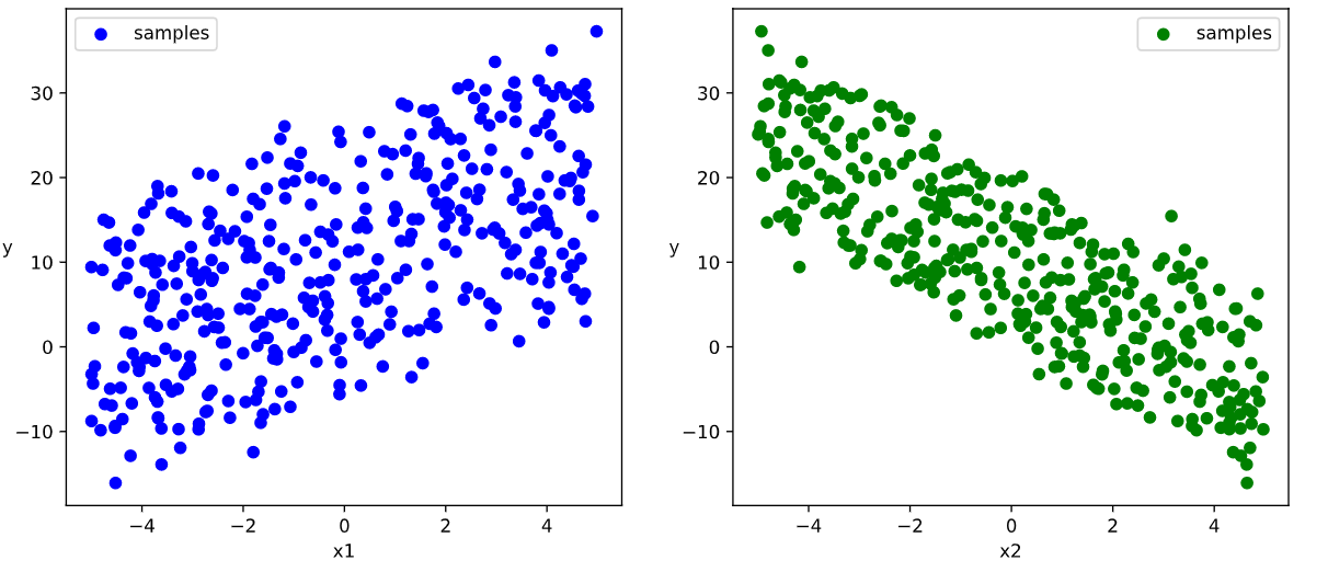
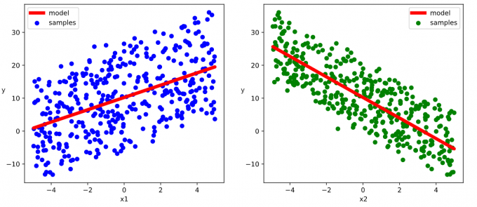
数据可视化
1
2
3
4
5
6
7
8
9
10
11
12
13
14
15
16
17
18# 数据可视化
%matplotlib inline
%config InlineBackend.figure_format = 'svg'
plt.figure(figsize = (12,5))
ax1 = plt.subplot(121)
ax1.scatter(X[:,0].numpy(),Y[:,0].numpy(), c = "b",label = "samples")
ax1.legend()
plt.xlabel("x1")
plt.ylabel("y",rotation = 0)
ax2 = plt.subplot(122)
ax2.scatter(X[:,1].numpy(),Y[:,0].numpy(), c = "g",label = "samples")
ax2.legend()
plt.xlabel("x2")
plt.ylabel("y",rotation = 0)
plt.show()Results:
构建数据管道迭代器
1
2
3
4
5
6
7
8
9
10
11
12
13
14# 构建数据管道迭代器
def data_iter(features, labels, batch_size=8):
num_examples = len(features)
indices = list(range(num_examples))
np.random.shuffle(indices) #样本的读取顺序是随机的
for i in range(0, num_examples, batch_size):
indexs = torch.LongTensor(indices[i: min(i + batch_size, num_examples)])
yield features.index_select(0, indexs), labels.index_select(0, indexs)
# 测试数据管道效果
batch_size = 8
(features,labels) = next(data_iter(X,Y,batch_size))
print(features)
print(labels)Result:
1
2
3
4
5
6
7
8
9
10
11
12
13
14
15
16tensor([[ 1.9428, -0.7624],
[-2.5625, 0.4411],
[-0.7651, -3.8922],
[ 3.1022, -2.6201],
[-1.0578, -2.6963],
[-1.9720, 3.8035],
[-3.4711, -2.4106],
[-0.6102, 2.6127]])
tensor([[11.7814],
[ 6.0209],
[23.4428],
[22.5369],
[17.8275],
[-8.7643],
[ 7.5050],
[ 0.5841]])
2.2 Model
2.2.1 Define model
1 | # 定义模型 |
2.2.2 Training model
1 | def train_step(model, features, labels): |
测试
train_step效果1
2
3batch_size = 10
(features,labels) = next(data_iter(X,Y,batch_size))
train_step(model,features,labels)Results:
1
tensor(68.6391, grad_fn=<MeanBackward0>)
Train model
1
2
3
4
5
6
7
8
9
10
11def train_model(model,epochs):
for epoch in range(1,epochs+1):
for features, labels in data_iter(X,Y,10):
loss = train_step(model,features,labels)
if epoch%200==0:
print("epoch =",epoch,"loss = ",loss.item())
print("model.w =",model.w.data)
print("model.b =",model.b.data)
train_model(model,epochs = 1000)Results:
1
2
3
4
5
6
7
8
9
10
11
12
13
14
15
16
17
18
19
20epoch = 200 loss = 3.2508397102355957
model.w = tensor([[ 2.0401],
[-2.9877]])
model.b = tensor([[9.9169]])
epoch = 400 loss = 3.0016872882843018
model.w = tensor([[ 2.0435],
[-2.9855]])
model.b = tensor([[9.9173]])
epoch = 600 loss = 2.7006335258483887
model.w = tensor([[ 2.0418],
[-2.9843]])
model.b = tensor([[9.9174]])
epoch = 800 loss = 1.280609369277954
model.w = tensor([[ 2.0416],
[-2.9869]])
model.b = tensor([[9.9169]])
epoch = 1000 loss = 2.169107675552368
model.w = tensor([[ 2.0420],
[-2.9852]])
model.b = tensor([[9.9170]])
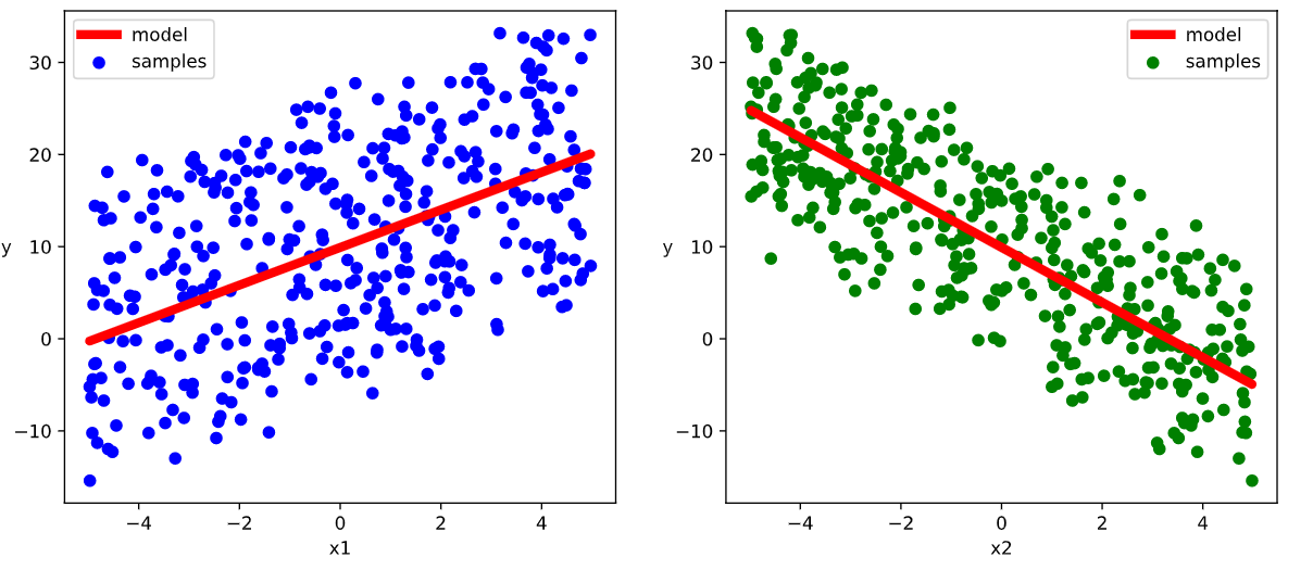
2.2.3 Visualization
1 | # 结果可视化 |
Results:
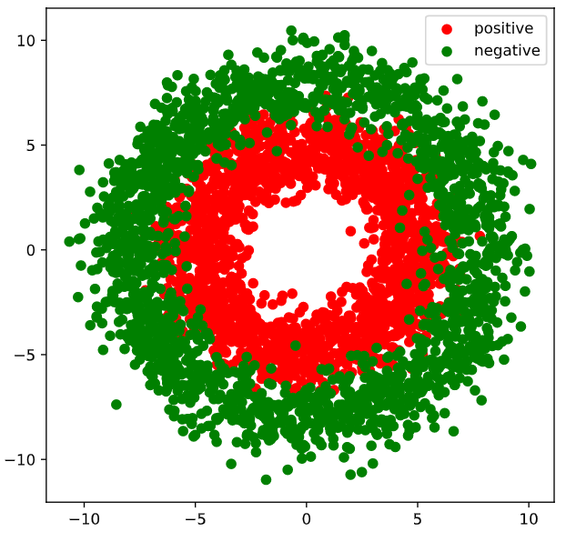
2.3 DNN二分类模型
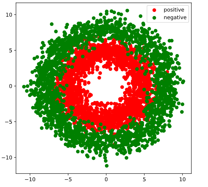
2.3.1 Prepare data
1 | import numpy as np |
Results:
构建数据管道迭代器
1
2
3
4
5
6
7
8
9
10
11
12
13
14
# 构建数据管道迭代器
def data_iter(features, labels, batch_size=8):
num_examples = len(features)
indices = list(range(num_examples))
np.random.shuffle(indices) #样本的读取顺序是随机的
for i in range(0, num_examples, batch_size):
indexs = torch.LongTensor(indices[i: min(i + batch_size, num_examples)])
yield features.index_select(0, indexs), labels.index_select(0, indexs)
# 测试数据管道效果
batch_size = 8
(features,labels) = next(data_iter(X,Y,batch_size))
print(features)
print(labels)Results:
1
2
3
4
5
6
7
8
9
10
11
12
13
14
15
16
tensor([[ 6.3216, -2.6834],
[ 2.4433, 4.4928],
[ 8.5585, 3.0958],
[-1.0328, 3.3381],
[-4.6885, -0.1144],
[ 8.7589, -3.4486],
[ 0.4830, 3.6482],
[ 4.9465, 0.3443]])
tensor([[0.],
[1.],
[0.],
[1.],
[1.],
[0.],
[1.],
[1.]])
2.3.2 Define model
此处范例我们利用 nn.Module 来组织模型变量。
1 | class DNNModel(nn.Module): |
测试模型结构
1
2
3
4
5
6
7
8
9
10
11# 测试模型结构
batch_size = 10
(features,labels) = next(data_iter(X,Y,batch_size))
predictions = model(features)
loss = model.loss_func(labels,predictions)
metric = model.metric_func(labels,predictions)
print("init loss:", loss.item())
print("init metric:", metric.item())Results:
1
2init loss: 7.446216583251953
init metric: 0.53620088100433351
len(list(model.parameters()))
Results:
1
6
2.3.3 Trianing model
1 | def train_step(model, features, labels): |
Results:
epoch = 100 loss = 0.1934373697731644 metric = 0.9207499933242798
epoch = 200 loss = 0.18901969484053552 metric = 0.918999993801117
epoch = 300 loss = 0.18451461097225547 metric = 0.9247499924898147
epoch = 400 loss = 0.18301934767514466 metric = 0.9247499933838844
epoch = 500 loss = 0.18300161071121693 metric = 0.9274999922513962
epoch = 600 loss = 0.18265636594966053 metric = 0.9219999933242797
epoch = 700 loss = 0.18221229410730302 metric = 0.9239999923110008
epoch = 800 loss = 0.1817048901133239 metric = 0.922749992609024
epoch = 900 loss = 0.18160937033127994 metric = 0.9259999924898148
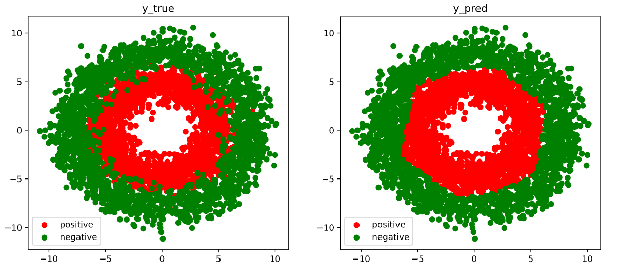
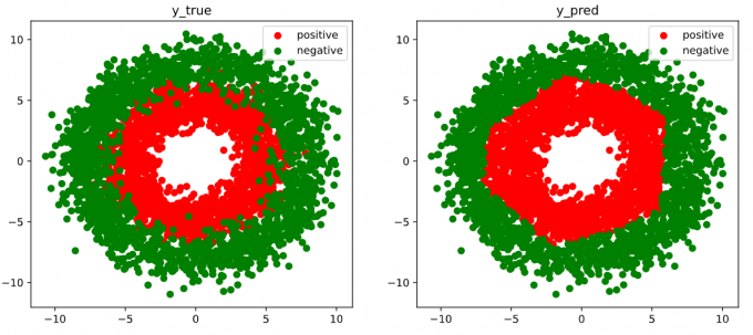
epoch = 1000 loss = 0.1799963693227619 metric = 0.92824999272823342.3.4 Visualization
1 | # 结果可视化 |
Results:
3. 中阶API示范
下面的范例使用 Pytorch 的中阶 API
实现线性回归模型和和 DNN 二分类模型。
Pytorch 的中阶 API 主要包括:
- 各种模型层;
- 损失函数;
- 优化器;
- 数据管道等。
3.1 Linear regression
3.1.1 Prepare data
1 | import numpy as np |
Visualization
1
2
3
4
5
6
7
8
9
10
11
12
13
14
15
16
17
18# 数据可视化
%matplotlib inline
%config InlineBackend.figure_format = 'svg'
plt.figure(figsize = (12,5))
ax1 = plt.subplot(121)
ax1.scatter(X[:,0],Y[:,0], c = "b",label = "samples")
ax1.legend()
plt.xlabel("x1")
plt.ylabel("y",rotation = 0)
ax2 = plt.subplot(122)
ax2.scatter(X[:,1],Y[:,0], c = "g",label = "samples")
ax2.legend()
plt.xlabel("x2")
plt.ylabel("y",rotation = 0)
plt.show()Results:

Data pipeline
1
2
3#构建输入数据管道
ds = TensorDataset(X,Y)
dl = DataLoader(ds,batch_size = 10,shuffle=True,num_workers=2)
3.2 Model
3.2.1 Define model
1 | model = nn.Linear(2,1) #线性层 |
3.2.2 Training model
Train step
1
2
3
4
5
6
7
8
9
10
11
12def train_step(model, features, labels):
predictions = model(features)
loss = model.loss_func(predictions,labels)
loss.backward()
model.optimizer.step()
model.optimizer.zero_grad()
return loss.item()
# 测试train_step效果
features,labels = next(iter(dl))
train_step(model,features,labels)Results:
1
415.08831787109375
Train model
1
2
3
4
5
6
7
8
9
10
11
12def train_model(model,epochs):
for epoch in range(1,epochs+1):
for features, labels in dl:
loss = train_step(model,features,labels)
if epoch%50==0:
w = model.state_dict()["weight"]
b = model.state_dict()["bias"]
print("epoch =",epoch,"loss = ",loss)
print("w =",w)
print("b =",b)
train_model(model,epochs = 200)Results:
1
2
3
4
5
6
7
8
9
10
11
12epoch = 50 loss = 4.598311901092529
w = tensor([[ 1.9602, -2.9793]])
b = tensor([10.1778])
epoch = 100 loss = 3.397813320159912
w = tensor([[ 2.0284, -2.9681]])
b = tensor([10.2230])
epoch = 150 loss = 1.588686227798462
w = tensor([[ 1.9387, -2.9690]])
b = tensor([10.1770])
epoch = 200 loss = 4.254576206207275
w = tensor([[ 1.8670, -3.1228]])
b = tensor([10.2100])
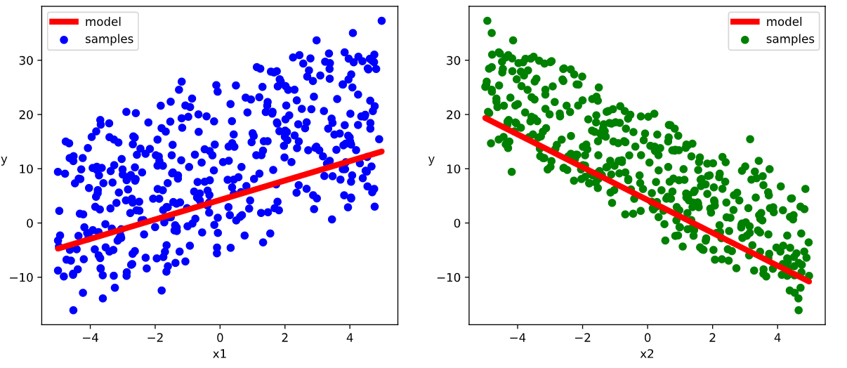
3.2.3 Visualization
1 | w,b = model.state_dict()["weight"],model.state_dict()["bias"] |
Results:
3.3 DNN二分类模型
3.3.1 Prepare data
1 | import numpy as np |
Results:
- Pipeline
1 | #构建输入数据管道 |
3.3.2 Define model
1 | class DNNModel(nn.Module): |
Test pipeline
1
2
3
4
5
6
7
8
9# 测试模型结构
(features,labels) = next(iter(dl))
predictions = model(features)
loss = model.loss_func(predictions,labels)
metric = model.metric_func(predictions,labels)
print("init loss:",loss.item())
print("init metric:",metric.item())Results:
1
2init loss: 0.8217536807060242
init metric: 0.6000000238418579
3.3.3 Training model
Train step
1
2
3
4
5
6
7
8
9
10
11
12
13
14
15
16
17
18
19def train_step(model, features, labels):
# 正向传播求损失
predictions = model(features)
loss = model.loss_func(predictions,labels)
metric = model.metric_func(predictions,labels)
# 反向传播求梯度
loss.backward()
# 更新模型参数
model.optimizer.step()
model.optimizer.zero_grad()
return loss.item(),metric.item()
# 测试train_step效果
features,labels = next(iter(dl))
train_step(model,features,labels)Results:
1
(1.027471899986267, 0.4000000059604645)
Train model
1
2
3
4
5
6
7
8
9
10
11
12
13
14def train_model(model,epochs):
for epoch in range(1,epochs+1):
loss_list,metric_list = [],[]
for features, labels in dl:
lossi,metrici = train_step(model,features,labels)
loss_list.append(lossi)
metric_list.append(metrici)
loss = np.mean(loss_list)
metric = np.mean(metric_list)
if epoch%100==0:
print("epoch =",epoch,"loss = ",loss,"metric = ",metric)
train_model(model,epochs = 300)Results:
1
2
3epoch = 100 loss = 0.2738241909684248 metric = 0.9302499929070472
epoch = 200 loss = 0.27702247152624065 metric = 0.9312499925494194
epoch = 300 loss = 0.27914922587944946 metric = 0.9309999929368495
3.3.4 Visualization
1 | # 结果可视化 |
Results:
4. 高阶API示范
Pytorch 没有官方的高阶
API,一般需要用户自己实现训练循环、验证循环、和预测循环。
torchkeras.Model 类是仿照 tf.keras.Model
的功能对 Pytorch 的 nn.Module
进行了封装设计而成的,它实现了 fit,
validate,predict, summary
方法,相当于用户自定义高阶
API。本章后面的内容借助它来实现线性回归模型。
此外,torchkeras.LightModel 类是借用
pytorch_lightning 的功能,封装了类Keras
接口的另外一种实现。本章后面的内容用它实现DNN二分类模型。
4.1 Linear regression
4.1.1 Prepare data
1 | import numpy as np |
Visualization
1
2
3
4
5
6
7
8
9
10
11
12
13
14
15
16
17
18# 数据可视化
%matplotlib inline
%config InlineBackend.figure_format = 'svg'
plt.figure(figsize = (12,5))
ax1 = plt.subplot(121)
ax1.scatter(X[:,0],Y[:,0], c = "b",label = "samples")
ax1.legend()
plt.xlabel("x1")
plt.ylabel("y",rotation = 0)
ax2 = plt.subplot(122)
ax2.scatter(X[:,1],Y[:,0], c = "g",label = "samples")
ax2.legend()
plt.xlabel("x2")
plt.ylabel("y",rotation = 0)
plt.show()Results:
Data pipeline
1
2
3
4
5#构建输入数据管道
ds = TensorDataset(X,Y)
ds_train,ds_valid = torch.utils.data.random_split(ds,[int(400*0.7),400-int(400*0.7)])
dl_train = DataLoader(ds_train,batch_size = 10,shuffle=True,num_workers=2)
dl_valid = DataLoader(ds_valid,batch_size = 10,num_workers=2)
4.2 Model
4.2.1 Define model
1 | # 继承用户自定义模型 |
4.2.2 Training model
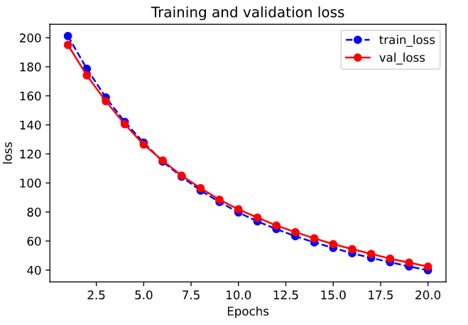
1 | # 使用fit方法进行训练 |
Results:
Start Training ...
================================================================================2022-02-06 22:48:10
{'step': 20, 'loss': 208.126, 'mae': 11.994, 'mape': 1.195}
+-------+---------+--------+-------+----------+---------+----------+
| epoch | loss | mae | mape | val_loss | val_mae | val_mape |
+-------+---------+--------+-------+----------+---------+----------+
| 1 | 201.175 | 11.695 | 1.269 | 195.057 | 11.834 | 1.065 |
+-------+---------+--------+-------+----------+---------+----------+
...
+-------+-------+-------+-------+----------+---------+----------+
| epoch | loss | mae | mape | val_loss | val_mae | val_mape |
+-------+-------+-------+-------+----------+---------+----------+
| 20 | 39.91 | 5.993 | 1.649 | 42.392 | 6.193 | 1.032 |
+-------+-------+-------+-------+----------+---------+----------+
================================================================================2022-02-06 22:49:56
Finished Training...4.2.3 Visualization
1 | w,b = model.state_dict()["fc.weight"],model.state_dict()["fc.bias"] |
Results:
4.2.4 Evaluation
1 | dfhistory.tail() |
Results:
| loss | mae | mape | val_loss | val_mae | val_mape | |
|---|---|---|---|---|---|---|
| 15 | 51.618867 | 6.840317 | 1.773152 | 54.423827 | 7.038455 | 1.124349 |
| 16 | 48.355738 | 6.618555 | 1.744567 | 51.134396 | 6.821975 | 1.102371 |
| 17 | 45.444238 | 6.420669 | 1.726280 | 47.896852 | 6.605719 | 1.086570 |
| 18 | 42.519069 | 6.199411 | 1.682794 | 45.115399 | 6.398358 | 1.055073 |
| 19 | 39.909953 | 5.992503 | 1.649152 | 42.391730 | 6.192853 | 1.031992 |
1 | import matplotlib.pyplot as plt |
Results:
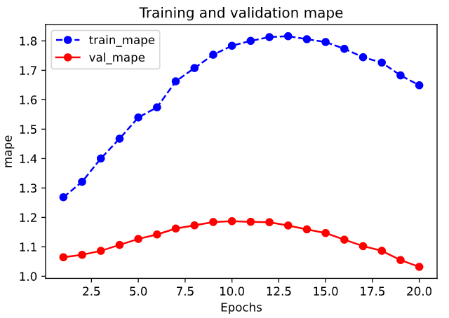
1 | plot_metric(dfhistory,"mape") |
Results:
1 | # 评估 |
Results:
{'val_loss': 42.391730308532715,
'val_mae': 6.19285261631012,
'val_mape': 1.0319924702246983}4.2.5 Predict
1 | # 预测 |
Results:
tensor([[ 8.9128],
[ 9.5116],
[ 12.2481],
[ 0.1308],
[ 16.1116],
[-17.9351],
[-14.6407],
[ 2.9675],
[ 10.9686],
[ 14.8227]])Predict validate data
1
2# 预测
model.predict(dl_valid)[0:10]Results:
tensor([[ -4.9393], [-12.2253], [ 3.5050], [ 6.6128], [ 2.7707], [ 0.7076], [ -6.2700], [ -8.4491], [ -7.4038], [ 10.0306]])
4.3 DNN二分类模型
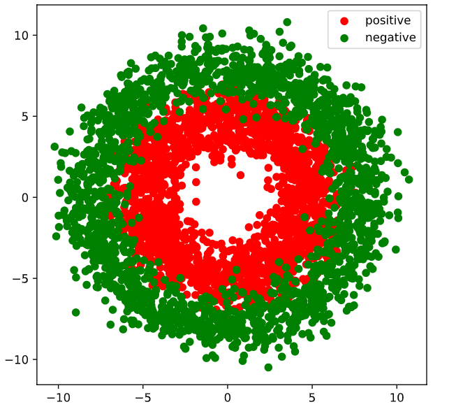
4.3.1 Prepare data
1 | import numpy as np |
Results:
Dataloader
1
2
3
4
5ds = TensorDataset(X,Y)
ds_train,ds_valid = torch.utils.data.random_split(ds,[int(len(ds)*0.7),len(ds)-int(len(ds)*0.7)])
dl_train = DataLoader(ds_train,batch_size = 100,shuffle=True,num_workers=2)
dl_valid = DataLoader(ds_valid,batch_size = 100,num_workers=2)
4.3.2 Define model
1 | import torchmetrics as metrics |
Results:
Global seed set to 1234

----------------------------------------------------------------
        Layer (type)               Output Shape         Param #
================================================================
            Linear-1                    [-1, 4]              12
            Linear-2                    [-1, 8]              40
            Linear-3                    [-1, 1]               9
================================================================
Total params: 61
Trainable params: 61
Non-trainable params: 0
----------------------------------------------------------------
Input size (MB): 0.000008
Forward/backward pass size (MB): 0.000099
Params size (MB): 0.000233
Estimated Total Size (MB): 0.000340
----------------------------------------------------------------
4.3.3 Training model
Note:下述代码,如果本机没有 gpu 会报
Runerror 错误:
1 | RuntimeError: DataLoader worker (pid(s) 6088, 19424) exited unexpectedl |
将 gpu=0 删掉能避免此错误。
1 | ckpt_cb = pl.callbacks.ModelCheckpoint(monitor='val_loss') |
Results:
1 | GPU available: False, used: False |
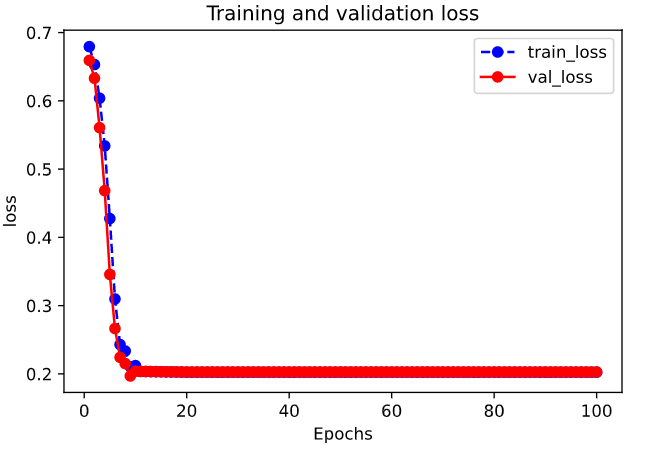
4.3.4 Visualization
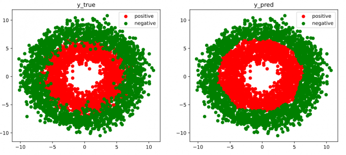
1 | # 结果可视化 |
Results:
4.3.5 Evaluation
1 | import pandas as pd |
Results:
| val_loss | val_acc | loss | acc | epoch | |
|---|---|---|---|---|---|
| 0 | 0.659258 | 0.548333 | 0.679371 | 0.532500 | 0 |
| 1 | 0.633105 | 0.712500 | 0.653128 | 0.617500 | 1 |
| 2 | 0.560715 | 0.705833 | 0.603827 | 0.702857 | 2 |
| 3 | 0.468437 | 0.794167 | 0.533967 | 0.737143 | 3 |
| 4 | 0.345662 | 0.820000 | 0.427476 | 0.795357 | 4 |
| ... | ... | ... | ... | ... | ... |
| 95 | 0.202806 | 0.918333 | 0.202421 | 0.921071 | 95 |
| 96 | 0.202806 | 0.918333 | 0.202421 | 0.921071 | 96 |
| 97 | 0.202806 | 0.918333 | 0.202421 | 0.921071 | 97 |
| 98 | 0.202806 | 0.918333 | 0.202421 | 0.921071 | 98 |
| 99 | 0.202806 | 0.918333 | 0.202421 | 0.921071 | 99 |
100 rows × 5 columns
1 | import matplotlib.pyplot as plt |
Results:
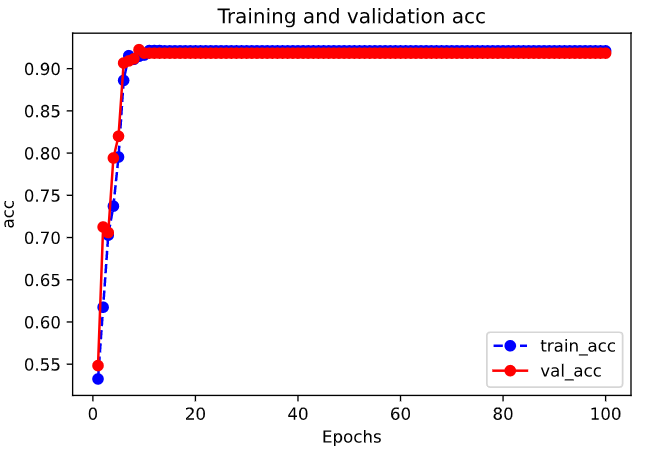
1 | plot_metric(dfhistory,"acc") |
Results:
1 | results = trainer.test(model, test_dataloaders=dl_valid, verbose = False) |
Results:
1 | Testing: 0it [00:00, ?it/s] |
4.3.6 Predict
1 | def predict(model,dl): |
Results:
tensor([[1.],
        [1.],
        [0.],
        ...,
        [0.],
        [0.],
        [1.]])