DataAnalysis-Modeling

1 Modeling creation

经过前面的学习，已可以对数数据进行增删查补和清洗工作。接下来需要使用处理好的数据进行分析和建模。这一章要做的是运用数据来得到某些结果。

分析的第一步是搭建一个预测模型或者其他；根据模型的结果，可以分析该模型是否可靠。

1.1 Preparation

• Import modules

  import pandas as pd
  import numpy as np
  import matplotlib.pyplot as plt
  import seaborn as sns
  from IPython.display import Image
  
  %matplotlib inline
  
  plt.rcParams['font.sans-serif'] = ['SimHei']  # 用来正常显示中文标签
  plt.rcParams['axes.unicode_minus'] = False  # 用来正常显示负号
  plt.rcParams['figure.figsize'] = (10, 6)  # 设置输出图片大小

• Load data

  # 读取原数据数集
  train = pd.read_csv('train.csv')
  train.shape
  
  #读取清洗过的数据集
  data = pd.read_csv('clear_data.csv')

1.2 Feature engineer

1.2.1 Fillna

• 对分类变量缺失值：填充某个缺失值字符(NA)、用最多类别的进行填充

  >>> train['Cabin'] = train['Cabin'].fillna('NA')
      train['Embarked'] = train['Embarked'].fillna('S')

• 对连续变量缺失值：填充均值、中位数、众数

  >>> train['Age'] = train['Age'].fillna(train['Age'].mean())

• 检查缺失值比例

  >>> train.isnull().sum().sort_values(ascending=False)
  
  PassengerId    0
  Survived       0
  Pclass         0
  Name           0
  Sex            0
  Age            0
  SibSp          0
  Parch          0
  Ticket         0
  Fare           0
  Cabin          0
  Embarked       0
  dtype: int64

1.2.2 Encoding classification variable

• 取出所有输入特征

  >>> data = train[['Pclass','Sex','Age','SibSp','Parch', 'Fare', 'Embarked']]

• 虚拟变量转换

  >>> data = pd.get_dummies(data)
      data.head()

  	Pclass	Age	SibSp	Parch	Fare	Sex_female	Sex_male	Embarked_C	Embarked_Q	Embarked_S
  0	3	22.0	1	0	7.2500	0	1	0	0	1
  1	1	38.0	1	0	71.2833	1	0	1	0	0
  2	3	26.0	0	0	7.9250	1	0	0	0	1
  3	1	35.0	1	0	53.1000	1	0	0	0	1
  4	3	35.0	0	0	8.0500	0	1	0	0	1

1.3 Construction

• 处理完数据的下一步是选择合适模型
• 在进行模型选择前，需要对数据集进行学习的方式是 监督学习 还是 无监督学习
• 模型的选择通过任务决定
• 除了根据们任务来选择模型，还可以根据数据样本量以及特征的稀疏性来决定
• 一般通常会尝试使用一个基本的模型来作为其 baseline，进而再训练其他模型做对比，最终选择泛化能力或性能比较好的模型

可以使用机器学习最常用的一个库 sklearn 来完成模型的搭建，sklearn 算法的选择路径如下：

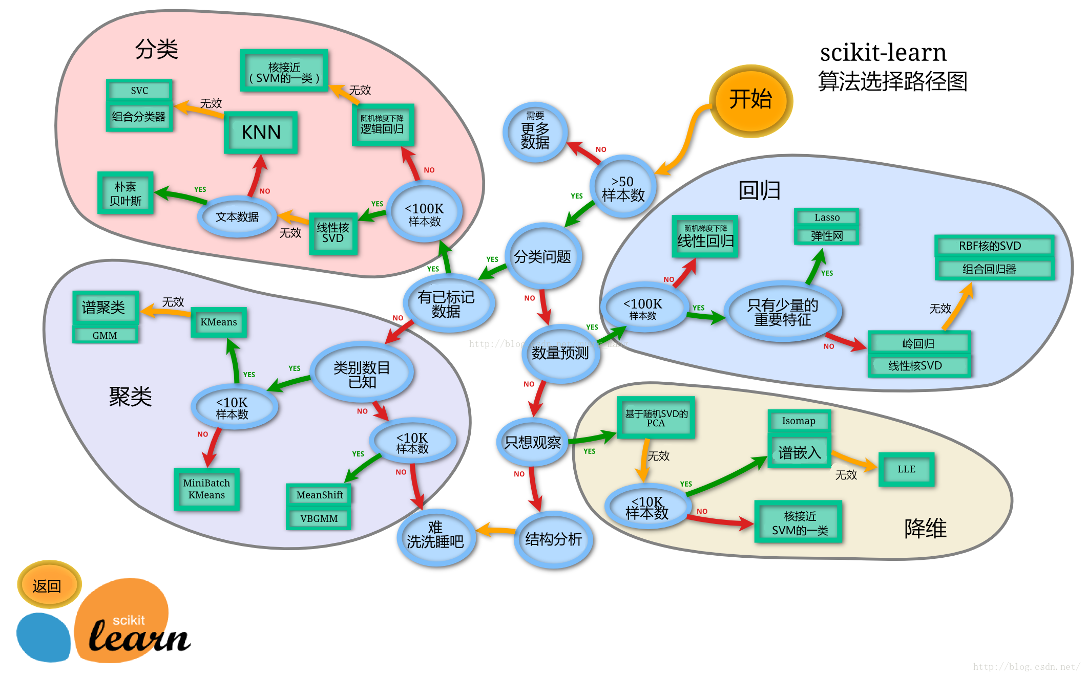
Note: 图源：莫凡Python-选择学习方法，如果想深入学习机器学习的话，也可关注该博客网站，上面有各大常用机器学习库的讲解视频的笔记，视频发布在 B 站莫烦Python 上，附几个热门的模块：

• Matplotlib
• Scikit-learn (sklearn)
• Pytorch 神经网络
• Keras

1.3.1 Split data

• 按比例切割数据集(常有30%、25%、20%、15%和10%)
• 按目标变量分层进行等比切割
• 设置随机种子以便结果能复现

Note:

• 切割数据集是为了后续评估模型泛化能力
• 查看函数文档可以在 notebook 里面使用 train_test_split? 和 help(train_test_split) 后回车即可看到
• 分层和随机种子在参数里寻找

>>> from sklearn.model_selection import train_test_split

    X = data.astype('float64')
    y = train['Survived'].astype('float64')

    X_train, X_test, y_train, y_test = train_test_split(X, y, stratify=y, random_state=0)

• 查看数据形状

>>> X_train.shape, X_test.shape

((668, 10), (223, 10))

1.3.2 Modeling

• 创建基于线性模型的分类模型（逻辑回归）
• 创建基于树的分类模型（决策树、随机森林）
• 查看模型的参数，并更改参数值，观察模型变化

Note:

• 逻辑回归不是回归模型而是 分类模型，不要与LinearRegression 混淆
• 随机森林其实是决策树集成为了降低决策树过拟合的情况
• 线性模型所在的模块为 sklearn.linear_model
• 树模型所在的模块为 sklearn.ensemble

线性模型的处理逻辑: 线性函数可以将平面进行分割，就形成了二分类问题。多分类的处理逻辑类似于线性规划，将平面分割为一个个小块。

1.3.3 Cases

本小节使用支持向量机和随即森林两个模型进行模型构建。

• 支持向量机

  >>> from sklearn.svm import SVCfrom sklearn.ensemble import RandomForestClassifier
  
      clf = SVC(probability=True)
      clf.fit(X_train, y_train

  # 查看训练集和测试集score值
  >>> print("Training set score: {:.2f}".format(clf.score(X_train, y_train)))
      print("Testing set score: {:.2f}".format(clf.score(X_test, y_test)))
  
  Training set score: 0.70Testing set score: 0.64

• 随机森林

  # 默认参数的随机森林分类模型
  >>> rfc = RandomForestClassifier()
      rfc.fit(X_train, y_train)
  
  RandomForestClassifier()

  >>> print("Training set score: {:.2f}".format(rfc.score(X_train, y_train)))
      print("Testing set score: {:.2f}".format(rfc.score(X_test, y_test)))
  
  Training set score: 0.99Testing set score: 0.81

  对随机森林模型进行调参：

  # 调整参数后的随机森林分类模型
  >>> rfc2 = RandomForestClassifier(n_estimators=100, max_depth=5)
      rfc2.fit(X_train, y_train)
  
      print("Training set score: {:.2f}".format(rfc2.score(X_train, y_train)))
      print("Testing set score: {:.2f}".format(rfc2.score(X_test, y_test)))
  
  Training set score: 0.86Testing set score: 0.83

1.4 Prediction

一般监督模型在 sklearn 里面有个 predict 能输出预测标签，predict_proba 则可以输出标签概率。

>>> pred = clf.predict(X_train)
    pred[:10]

array([1., 0., 0., 0., 0., 0., 0., 1., 1., 1.])

• 预测概率

  >>> pred_proba = clf.predict_proba(X_train)
      pred_proba[:10]
  
  array([[0.43518882, 0.56481118],
         [0.68639392, 0.31360608],
         [0.62646492, 0.37353508],
         [0.62676837, 0.37323163],
         [0.70955025, 0.29044975],
         [0.72361218, 0.27638782],
         [0.64503542, 0.35496458],
         [0.38964073, 0.61035927],
         [0.23539098, 0.76460902],
         [0.26563197, 0.73436803]])

2 Model evaluation

根据之前的模型的建模，已经学会了运用 sklearn 库来完成建模，以及数据集的划分等操作。那么如何评估模型的优劣呢？以及如何判断模型给出的结果是否有效呢？这也是本次任务需要学习的内容。

2.1 Preparation

2.1.1 Load modules

from sklearn.linear_model import LogisticRegression
from sklearn.ensemble import RandomForestClassifier

%matplotlib inline

plt.rcParams['font.sans-serif'] = ['SimHei']  # 用来正常显示中文标签
plt.rcParams['axes.unicode_minus'] = False  # 用来正常显示负号
plt.rcParams['figure.figsize'] = (10, 6)  # 设置输出图片大小

2.1.2 Load data

一般先取出 X 和 y 后再切割，有些情况会使用到未切割的，这时候 X 和 y 就可以用，x 是清洗好的数据，y 是我们要预测的存活数据 Survived。

>>> data = pd.read_csv('clear_data.csv')
    train = pd.read_csv('train.csv')
    X = data.astype('float64')
    y = train['Survived'].astype('float64')

2.1.3 Split data

>>> from sklearn.model_selection import train_test_split

    # 对数据集进行切割
    X_train, X_test, y_train, y_test = train_test_split(X, y, stratify=y, random_state=0)

注意到，在本例子中使用了 stratify 参数，其目的是保持测试集与整个数据集里 y 的数据分类比例一致。

举个栗子： 如何整个数据集有 1000 行，y 列的数据也是 1000 个，而且分两类：0 和 1，其中 0 有 300 个，1 有 700 个，即数据分类的比例为 3：7。那么现在把整个数据 split，因为 test_size = 0.2，所以训练集分到 800 个数据，测试集分到 200 个数据。

重点：由于 stratify = y，则训练集和测试集中的数据分类比例将与 y 一致，也是 3：7，结果就是在训练集中，有 240 个 0 和 560 个 1；测试集中有 60 个 0 和 140 个 1 。

>>> y_train.values.shape

(668,)

2.2 Construction

• 拟合

  # 默认参数逻辑回归模型
  >>> clf = RandomForestClassifier()
      clf.fit(X_train.values, y_train)

• 预测

  >>> clf.predict(X_test)[:10]
  
  array([0., 1., 0., 0., 1., 0., 0., 0., 0., 0.])

2.3 Evaluation

• 模型评估是为了知道模型的泛化能力。
• 交叉验证（cross-validation）是一种评估泛化性能的统计学方法，它比单次划分训练集和测试集的方法更加稳定、全面。
• 在交叉验证中，数据被多次划分，并且需要训练多个模型。
• 最常用的交叉验证是 k 折交叉验证（k-fold cross-validation），其中 k 是由用户指定的数字，通常取 5 或 10。
• 准确率（Precision）度量的是被预测为正例的样本中有多少是真正的正例
• 召回率（Recall）度量的是正类样本中有多少被预测为正类
• f-分数是准确率与召回率的调和平均

2.3.1 Cross-validation

1. 概念

   交叉验证是建立模型和验证模型参数时常用的办法。顾名思义，就是重复的对样本数据进行切分，组合为不同的训练集和测试集，并用训练集来训练模型，用测试集来评估模型。

   在此基础上可以得到多组不同的训练集和测试集，某次训练集中的某样本在下次可能成为测试集中的样本，即所谓“交叉”。

2. 思考：那么什么时候才需要交叉验证呢？

   交叉验证常用在数据不是很充足时。如果数据样本量较小，可以采用交叉验证来训练优化选择模型。若样本充足，一般可把数据随机地分成三份：Training Set，Validation Set，Test Set。用 Training Set 来训练模型，用 Validation Set 来评估模型预测的好坏和选择模型及其对应的参数。把最终得到的模型再用于 Test Set ，最终决定使用哪个模型以及对应参数。

3. 常见形式：

   • Holdout

   常识来说，Holdout 验证并非一种交叉验证，因为数据并没有交叉使用。 随机从最初的样本中选出部分，形成交叉验证数据，而剩余的就当做训练数据。 一般来说，少于原本样本三分之一的数据被选做验证数据。

   • K-fold cross-validation:

   K 折交叉验证，初始采样分割成 K 个子样本，一个单独的子样本被保留作为验证模型的数据，其他 K-1 个样本用来训练。交叉验证重复K次，每个子样本验证一次，平均 K 次的结果或者使用其它结合方式，最终得到一个单一估测。这个方法的优势在于，同时重复运用随机产生的子样本进行训练和验证，每次的结果验证一次，10 折交叉验证是最常用的。5 折交叉验证的示例图如下：

   • Leave-one-out Cross Validation:

   留一验证（LOOCV）是 K 折交叉验证的特例，此时折数 K 等于原本样本个数。意指只使用原本样本中的一项来当做验证资料， 而剩余的则留下来当做训练资料。 这个步骤一直持续到每个样本都被当做一次验证资料。在某些情况下是存在有效率的演算法，如使用kernel regression 和 Tikhonov regularization。

   Note: 上述交叉验证的解释内容部分来自搜狗百科词条 交叉验证。

4. K 折交叉验证的使用

   在本节中主要介绍 K 折交叉验证的使用，借助 sklearn.model_selection 来实现利用 10 折交叉验证来评估前文的随机森林分类模型。

>>> from sklearn.model_selection import cross_val_score

    clf = RandomForestClassifier()
    scores = cross_val_score(clf, X_train, y_train, cv=10)

    # k折交叉验证分数
    scores

array([0.88059701, 0.80597015, 0.8358209 , 0.82089552, 0.7761194 ,
       0.8358209 , 0.8358209 , 0.80597015, 0.83333333, 0.8030303 ])

# 平均交叉验证分数
>>> print("Average cross-validation score: {:.2f}".format(scores.mean()))

Average cross-validation score: 0.82

折数越多代表着运行时间越长。

import timefrom sklearn.model_selection
import LeaveOneOut

# 10 折
start = time.time()
scores_fold = cross_val_score(clf, X_train, y_train, cv=10)
transition = time.time()

# 留一验证
loocv = LeaveOneOut()
scores_leave = cross_val_score(clf, X_train, y_train, cv=loocv)
end = time.time()

print('The 10-fold spend {:.2f}s, the leave one spend {:.2f}s'.format(
        transition-start, end-transition))
print("Average 10-fold cross-validation score: {:.2f}".format(scores.mean()))
print("Average leave-one-out cross-validation score: {:.2f}".format(scores.mean()))

The 10-fold spend 2.72s, the leave one spend 189.75s
Average 10-fold cross-validation score: 0.82
Average leave-one-out cross-validation score: 0.82

>>> print(len(y_train)/10)

66.8

>>> print(189.75/2.72)

69.7610294117647

可以发现采用 10 折仅费了 2.72s，而将折数上调至极限（留一验证）时，花费的时间几乎增加了了 70 倍，同时可以发现倍数与折数比几乎相同。

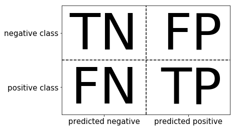
2.3.2 Confusion matrix

任务：

• 计算二分类问题的混淆矩阵
• 计算精确率、召回率以及f-分数

1. 混肴矩阵

   示意图如下：

   

2. 指标值

   准确率 Accuracy，精确度 Precision，Recall，f-score 的计算方式：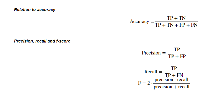

   

   • 混淆矩阵的方法在 sklearn.metrics 模块
   • 混淆矩阵需要输入真实标签和预测标签
   • Precision，Recall，f-score可以使用 classification_report 模块

from sklearn.metrics import confusion_matrix

clf = RandomForestClassifier()
clf.fit(X_train.values, y_train) # 训练

# 模型预测结果
pred = clf.predict(X_train)

混淆矩阵：

>>> confusion_matrix(y_train, pred)

array([[412,   0],
       [  0, 256]], dtype=int64)

指标值：

from sklearn.metrics import classification_report
print(classification_report(y_train, pred))

              precision    recall  f1-score   support

         0.0       1.00      1.00      1.00       412
         1.0       1.00      1.00      1.00       256

    accuracy                           1.00       668
   macro avg       1.00      1.00      1.00       668
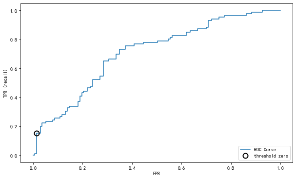
weighted avg       1.00      1.00      1.00       668

2.3.3 ROC curve

• ROC曲线在sklearn中的模块为sklearn.metrics
• ROC曲线下面所包围的面积越大越好

from sklearn.svm import SVC # 支持向量机
from sklearn.metrics import roc_curve

# clf = SVC(decision_function_shape="ovr",probability=True)
clf = SVC(probability=True)
clf.fit(X_train.values, y_train) # 训练

fpr, tpr, thresholds = roc_curve(y_test, clf.decision_function(X_test))
plt.plot(fpr, tpr, label="ROC Curve")
plt.xlabel("FPR")
plt.ylabel("TPR (recall)")

# 找到最接近于0的阈值
close_zero = np.argmin(np.abs(thresholds))
plt.plot(fpr[close_zero], tpr[close_zero], 'o', markersize=10,
         label="threshold zero", fillstyle="none", c='k', mew=2)
plt.legend(loc=4)

Result:

在上述使用的支持向量机中，对于 n 分类，会有 n 个分类器，然后，任意两个分类器都可以算出一个分类界面，这样，用 decision_function() 时，对于任意一个样例，就会有 \(n*(n-1)/2\) 个值。

任意两个分类器可以算出一个分类界面，然后这个值就是距离分类界面的距离。这个函数可能是为了统计画图，对于二分类时最明显，用来统计每个点离超平面有多远，为了在空间中直观的表示数据以及画超平面还有间隔平面等。 decision_function_shape 为 ovr 时是 4 个值，为 ovo 时是 6 个值。

>>> clf.decision_function(X_test)[:5]

array([-0.98942638, -0.96365727, -0.81459531, -0.64715413, -0.38873267])

• np.argmin()

  获取最小值索引位置。

  >>> np.argmin(np.abs(thresholds))
  
  4

• 计算得分

  >>> clf.predict_proba(X) #这个是得分,每个分类器的得分，取最大得分对应的类。
  
  array([[0.68136476, 0.31863524],
         [0.61321679, 0.38678321],
         [0.68211357, 0.31788643],
         			...,       
         [0.63577539, 0.36422461],
         [0.61380992, 0.38619008],
         [0.68829583, 0.31170417]])

2.3.4 Classification boundary

借助 decision_function 还在输入特征较少时直观地画出分类边界图。下面以一个输入特征为二维的小例子展示二维平面分类边界的绘制，案例参考自 胖大海瘦西湖的博文。

• 模型构建

  import matplotlib.pyplot as plt
  import numpy as np
  from sklearn.svm import SVC
  
  # 构建输入特征和输出特征
  X = np.array([[-1,-1],[-2,-1],[1,1],[2,1],[-1,1],[-1,2],[1,-1],[1,-2]])
  y = np.array([0,0,1,1,2,2,3,3])
  
  # clf = SVC(decision_function_shape="ovr",probability=True)
  clf = SVC(probability=True)
  clf.fit(X, y)

  plot_step=0.02
  x_min, x_max = X[:, 0].min() - 1, X[:, 0].max() + 1 # X 的第一维作为横坐标
  y_min, y_max = X[:, 1].min() - 1, X[:, 1].max() + 1 # 第二维作为纵坐标
  
  xx, yy = np.meshgrid(np.arange(x_min, x_max, plot_step),
                       np.arange(y_min, y_max, plot_step))
  
  # 对坐标风格上的点进行预测，来画分界面。其实最终看到的类的分界线就是分界面的边界线。
  Z = clf.predict(np.c_[xx.ravel(), yy.ravel()])
  Z = Z.reshape(xx.shape)

Note: 上述代码中使用到了 np.meshgrid 函数，官方文档看起来文绉绉的，理解起来不是很直观。通俗来讲，这个函数的作用是利用两个坐标轴上的点在平面上画网格。

返回两个参数，xx 中记录了网格中所有点的横坐标，yy 记录了网格中所有点的纵坐标。其运行过程可通过下图加深理解：

（图源公众号： Python数据之道）

用法：

• [X, Y] = meshgrid(x, y)
• [X, Y] = meshgrid(x)与 [X, Y] = meshgrid(x, x) 等同
• [X, Y, Z] = meshgrid(x, y, z) 生成三维数组，可用来计算三变量的函数和绘制三维立体图

cs = plt.contourf(xx, yy, Z, cmap=plt.cm.Paired) # 绘制轮廓线
plt.axis("tight")

class_names="ABCD"
plot_colors="rybg"
for i, n, c in zip(range(4), class_names, plot_colors):
    idx = np.where(y == i) #i为0或者1，两个类
    plt.scatter(X[idx, 0], X[idx, 1],
                c=c, cmap=plt.cm.Paired,
                label="Class %s" % n)

plt.xlim(x_min, x_max)
plt.ylim(y_min, y_max)
plt.legend(loc='upper right')
plt.xlabel('x')
plt.ylabel('y')
plt.title('Decision Boundary')
plt.show()

Results: