1. Problem

1.1 Introduction of Background

火力发电的基本原理是：颜料燃烧时加热水会生成蒸汽，蒸汽压力推动汽轮机旋转，然后汽轮机带动带动发电机旋转，产生电能。在这一系列的能量转化中，影响发电效率的核心是锅炉的燃烧效率，即燃料燃烧加热水产生高温高压蒸汽。锅炉的燃烧效率的影响因素很多，包括锅炉的可调参数，如燃烧给量，一二次风，引风，返料风，给水水量；以及锅炉的工况，比如锅炉床温、床压，炉膛温度、压力，过热器的温度等。我们如何使用以上的信息，根据锅炉的工况，预测产生的蒸汽量，来为我国的工业届的产量预测贡献自己的一份力量呢？

此次的案列时使用工业指标的特征，进行蒸汽量的预测。所使用的数据均为脱敏后的数据。

1.2 Data source

数据分成训练数据（train.txt）和测试数据（test.txt），其中字段 V0-V37，这 38 个字段是作为特征变量，target 作为目标变量。我们需要利用训练数据训练出模型，预测测试数据的目标变量。

数据包下载地址: Data of case。

1.3 Evaluation metrics

最终的评价指标为均方误差 \(MSE\) ，即： \(Score = \frac{1}{n}\sum^n_1 (y_i - y^*)^2\)

2. Data process

2.1 Load data

import pandas as pd

data_train = pd.read_csv('train.txt', sep = '\t')
data_test = pd.read_csv('test.txt', sep = '\t')

# concantenate
data_train['oringin'] = 'train'
data_test['oringin'] = 'test'
data_all = pd.concat([data_train, data_test], axis = 0, ignore_index = True)

查看合并后的数据信息：

1	data_all.head()

Result:

	V0	V1	V2	V3	V4	V5	V6	V7	V8	V9	...	V30	V31	V32	V33	V34	V35	V36	V37	target	oringin
0	0.566	0.016	-0.143	0.407	0.452	-0.901	-1.812	-2.360	-0.436	-2.114	...	0.109	-0.615	0.327	-4.627	-4.789	-5.101	-2.608	-3.508	0.175	train
1	0.968	0.437	0.066	0.566	0.194	-0.893	-1.566	-2.360	0.332	-2.114	...	0.124	0.032	0.600	-0.843	0.160	0.364	-0.335	-0.730	0.676	train
2	1.013	0.568	0.235	0.370	0.112	-0.797	-1.367	-2.360	0.396	-2.114	...	0.361	0.277	-0.116	-0.843	0.160	0.364	0.765	-0.589	0.633	train
3	0.733	0.368	0.283	0.165	0.599	-0.679	-1.200	-2.086	0.403	-2.114	...	0.417	0.279	0.603	-0.843	-0.065	0.364	0.333	-0.112	0.206	train
4	0.684	0.638	0.260	0.209	0.337	-0.454	-1.073	-2.086	0.314	-2.114	...	1.078	0.328	0.418	-0.843	-0.215	0.364	-0.280	-0.028	0.384	train

5 rows × 40 columns

2.2 Data exploration

2.2.1 EDA

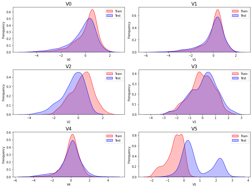
由于是传感器数据，所以这些变量都是连续便来给你，故使用 kdeplot（核密度估计图）进行数据的初步分析，即 EDA。

import matplotlib.pyplot as plt
import seaborn as sns

columns = data_all.columns[0:-2]

num_subfig = 6 # 每个大图中有多少小图
num_fig = len(columns) // num_subfig # 需要多少个大图

for i in range(num_fig):
    f = plt.figure(figsize = (12, 9))
    for j in range(num_subfig):
        column = columns[i*num_subfig+j]
        # ax = f.add_subplot(4, 3, j+1) # 当 num_subfit = 12 时使用
        ax = f.add_subplot(3, 2, j+1) # 当 num_subfit = 6 时使用
        sns.kdeplot(data_all[column][(data_all["oringin"] == "train")],
                    color="Red", shade = True)
        sns.kdeplot(data_all[column][(data_all["oringin"] == "test")],
                    ax = ax, color="Blue", shade= True)
        ax.set_title('V{}'.format(i*num_subfig+j), fontsize = 16)
        ax.set_xlabel(column)
        ax.set_ylabel('Frenquency')
        ax.legend(['Train', 'Test'])
    plt.tight_layout()
    plt.show()

for i in range(2):
    f = plt.figure(figsize = (12, 3))
    column = columns[36+i]
    ax = f.add_subplot(1, 2, i+1)
    sns.kdeplot(data_all[column][(data_all["oringin"] == "train")],
                color="Red", shade = True)
    sns.kdeplot(data_all[column][(data_all["oringin"] == "test")],
                ax = ax, color="Blue", shade= True)
    ax.set_title('V{}'.format(36+i), fontsize = 16)
    ax.set_xlabel(column)
    ax.set_ylabel('Frenquency')
    ax.legend(['Train', 'Test'])
plt.tight_layout()
plt.show()

Delete variables

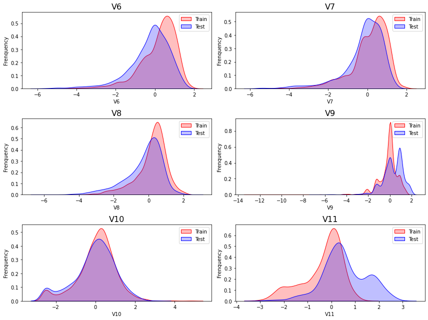
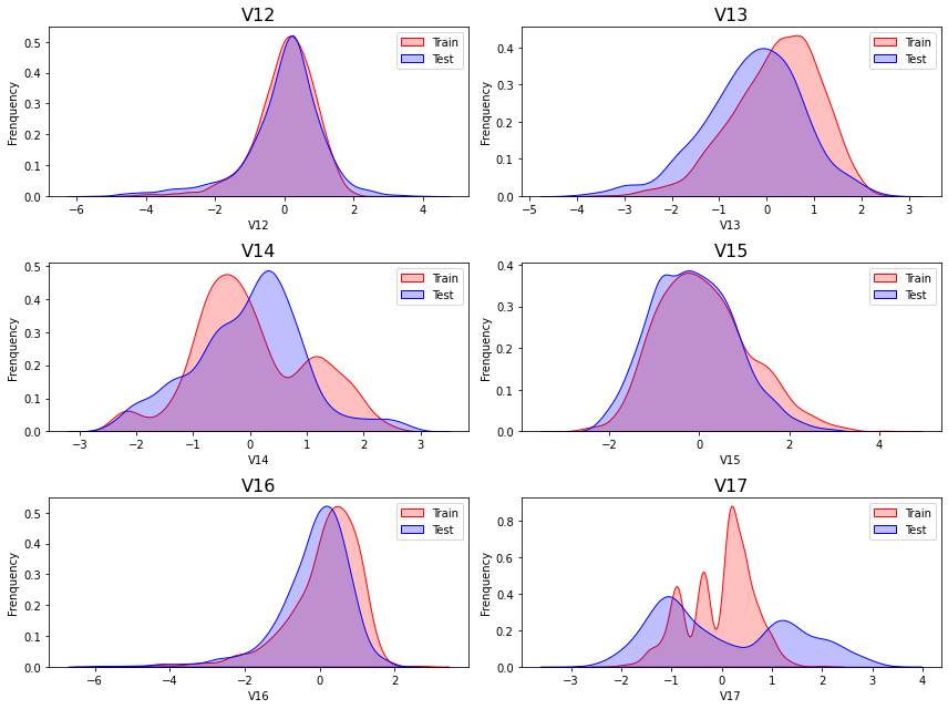
从上述的图中可以看出，特征征 V5, V9, V11, V17, V22, V28中的训练集数据分布和测试集数据分布分布不均，所以我们删除这些特则会给你数据。

f = plt.figure(figsize = (12, 9))

drop_columns = ['V5', 'V9', 'V11', 'V17', 'V22', 'V28']
for i in range(6):
    column = drop_columns[i]
    # ax = f.add_subplot(4, 3, j+1) # 当 num_subfit = 12 时使用
    ax = f.add_subplot(3, 2, i+1) # 当 num_subfit = 6 时使用
    sns.kdeplot(data_all[column][(data_all["oringin"] == "train")],
                color="Red", shade = True)
    sns.kdeplot(data_all[column][(data_all["oringin"] == "test")],
                ax = ax, color="Blue", shade= True)
    ax.set_title(column, fontsize = 16)
    ax.set_xlabel(column)
    ax.set_ylabel('Frenquency')
    ax.legend(['Train', 'Test'])
plt.tight_layout()
plt.show()

data_all.drop(["V5","V9","V11","V17","V22","V28"],axis=1,inplace=True)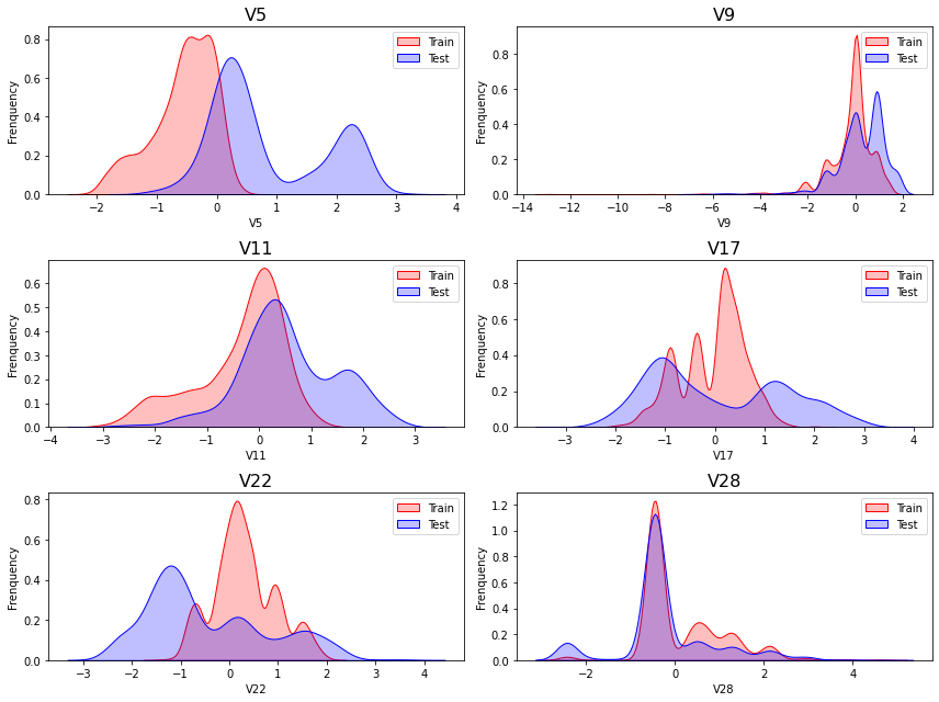

2.2.2 Dimentsionality

import numpy as np

data_train1 = data_all[data_all["oringin"]=="train"].drop("oringin",axis=1)
plt.figure(figsize=(20, 16)) # 指定绘图对象宽度和高度
colnm = data_train1.columns.tolist() # 列表头
mcorr = data_train1[colnm].corr(method="spearman") # 相关系数矩阵，即给出了任意两个变量之间的相关系数
mask = np.zeros_like(mcorr, dtype=np.bool) # 构造与mcorr同维数矩阵 为bool型
mask[np.triu_indices_from(mask)] = True # 角分线右侧为True
cmap = sns.diverging_palette(220, 10, as_cmap=True) # 返回matplotlib colormap对象，调色板
g = sns.heatmap(mcorr, mask=mask, cmap=cmap, square=True, annot=True, fmt='0.2f') # 热力图（看两两相似度）
plt.show()

降维操作

可以发现部分特征 (V14, V21, V22, V25, V26, V32, V33, V34, V35) 与 target 的相关性非常小，其中可能包含几乎很少的对target 的预测信息，因此，对这些变量进行剔除。
1
2
3
4
threshold = 0.1
corr_matrix = data_train1.corr().abs()
drop_col=corr_matrix[corr_matrix["target"]<threshold].index
data_all.drop(drop_col,axis=1,inplace=True)

Normalization

cols_numeric = list(data_all.columns)
cols_numeric.remove('oringin')
def scale_minmax(col):
    return (col - col.min())/(col.max()-col.min())
scale_cols = [col for col in cols_numeric if col != 'target']
data_all[scale_cols] = data_all[scale_cols].apply(scale_minmax,axis=0)
data_all[scale_cols].describe()

	V0	V1	V2	V3	V4	V6	V7	V8	V10	V12	...	V20	V23	V24	V27	V29	V30	V31	V35	V36	V37
count	4813.000000	4813.000000	4813.000000	4813.000000	4813.000000	4813.000000	4813.000000	4813.000000	4813.000000	4813.000000	...	4813.000000	4813.000000	4813.000000	4813.000000	4813.000000	4813.000000	4813.000000	4813.000000	4813.000000	4813.000000
mean	0.694172	0.721357	0.602300	0.603139	0.523743	0.748823	0.745740	0.715607	0.348518	0.578507	...	0.456147	0.744438	0.356712	0.881401	0.388683	0.589459	0.792709	0.762873	0.332385	0.545795
std	0.144198	0.131443	0.140628	0.152462	0.106430	0.132560	0.132577	0.118105	0.134882	0.105088	...	0.134083	0.134085	0.265512	0.128221	0.133475	0.130786	0.102976	0.102037	0.127456	0.150356
min	0.000000	0.000000	0.000000	0.000000	0.000000	0.000000	0.000000	0.000000	0.000000	0.000000	...	0.000000	0.000000	0.000000	0.000000	0.000000	0.000000	0.000000	0.000000	0.000000	0.000000
25%	0.626676	0.679416	0.514414	0.503888	0.478182	0.683324	0.696938	0.664934	0.284327	0.532892	...	0.370475	0.719362	0.040616	0.888575	0.292445	0.550092	0.761816	0.727273	0.270584	0.445647
50%	0.729488	0.752497	0.617072	0.614270	0.535866	0.774125	0.771974	0.742884	0.366469	0.591635	...	0.447305	0.788817	0.381736	0.916015	0.375734	0.594428	0.815055	0.800020	0.347056	0.539317
75%	0.790195	0.799553	0.700464	0.710474	0.585036	0.842259	0.836405	0.790835	0.432965	0.641971	...	0.522660	0.792706	0.574728	0.932555	0.471837	0.650798	0.852229	0.800020	0.414861	0.643061
max	1.000000	1.000000	1.000000	1.000000	1.000000	1.000000	1.000000	1.000000	1.000000	1.000000	...	1.000000	1.000000	1.000000	1.000000	1.000000	1.000000	1.000000	1.000000	1.000000	1.000000

8 rows × 25 columns

2.3.3 Features engineering

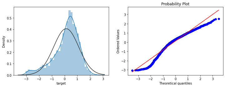
绘图显示 Box-Cox 变换对数据分布影响，Box-Cox 用于连续的响应变量不满足正态分布的情况。在进行 Box-Cox 变换之后，可以一定程度上减少不可观测的误差和预测变量的相关性。

quantitle-quantile(q-q) 图，可参考 QQ图，stats.probplot

import warnings
warnings.filterwarnings("ignore")
from scipy import stats

fcols = 6
frows = len(cols_numeric)-1
plt.figure(figsize=(4*fcols,4*frows))
i=0

for var in cols_numeric:
    if var!='target':
        dat = data_all[[var, 'target']].dropna()

        i+=1
        plt.subplot(frows,fcols,i)
        sns.distplot(dat[var] , fit=stats.norm);
        plt.title(var+' Original')
        plt.xlabel('')

        i+=1
        plt.subplot(frows,fcols,i)
        _=stats.probplot(dat[var], plot=plt)
        plt.title('skew='+'{:.4f}'.format(stats.skew(dat[var])))
        plt.xlabel('')
        plt.ylabel('')

        i+=1
        plt.subplot(frows,fcols,i)
        plt.plot(dat[var], dat['target'],'.',alpha=0.5)
        plt.title('corr='+'{:.2f}'.format(np.corrcoef(dat[var], dat['target'])[0][1]))

        i+=1
        plt.subplot(frows,fcols,i)
        trans_var, lambda_var = stats.boxcox(dat[var].dropna()+1)
        trans_var = scale_minmax(trans_var)
        sns.distplot(trans_var , fit=stats.norm);
        plt.title(var+' Tramsformed')
        plt.xlabel('')

        i+=1
        plt.subplot(frows,fcols,i)
        _=stats.probplot(trans_var, plot=plt)
        plt.title('skew='+'{:.4f}'.format(stats.skew(trans_var)))
        plt.xlabel('')
        plt.ylabel('')

        i+=1
        plt.subplot(frows,fcols,i)
        plt.plot(trans_var, dat['target'],'.',alpha=0.5)
        plt.title('corr='+'{:.2f}'.format(np.corrcoef(trans_var,dat['target'])[0][1]))

Box-Cox 变换

# 进行Box-Cox变换
cols_transform=data_all.columns[0:-2]
for col in cols_transform:
    # transform column
    data_all.loc[:,col], _ = stats.boxcox(data_all.loc[:,col]+1)
print(data_all.target.describe())
plt.figure(figsize=(12,4))
plt.subplot(1,2,1)
sns.distplot(data_all.target.dropna() , fit=stats.norm);
plt.subplot(1,2,2)
_=stats.probplot(data_all.target.dropna(), plot=plt)

Results:

count    2888.000000
mean        0.126353
std         0.983966
min        -3.044000
25%        -0.350250
50%         0.313000
75%         0.793250
max         2.538000
Name: target, dtype: float64

对数变换 target

使用对数变换 target 目标提升特征数量的正态性，可以参考知乎文章：在统计学中为什么要对变量取对数？

sp = data_train.target
data_train.target1 = np.power(1.5,sp)
print(data_train.target1.describe())

plt.figure(figsize=(12,4))
plt.subplot(1,2,1)
sns.distplot(data_train.target1.dropna(),fit=stats.norm);
plt.subplot(1,2,2)
_ = stats.probplot(data_train.target1.dropna(), plot=plt)

Results:

count    2888.000000
mean        1.129957
std         0.394110
min         0.291057
25%         0.867609
50%         1.135315
75%         1.379382
max         2.798463
Name: target, dtype: float64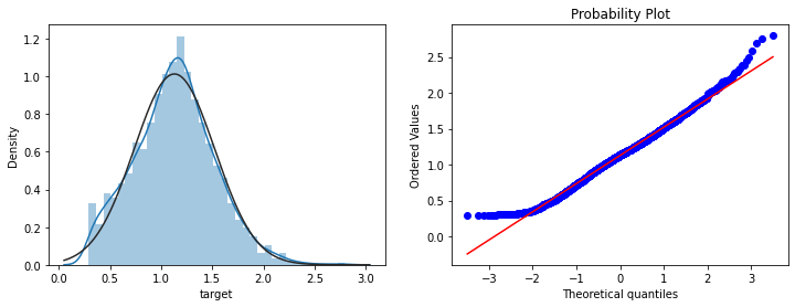

3. Model construction

3.1 Self definition fuction

Train set and Test set

from sklearn.model_selection import train_test_split

# function to get training samples
def get_training_data():
    # extract training samples
    df_train = data_all[data_all["oringin"]=="train"]
    df_train["label"] = data_train.target1
    # split SalePrice and features
    y = df_train.target
    X = df_train.drop(["oringin","target","label"], axis=1)
    X_train,X_valid,y_train,y_valid=train_test_split(X,
                        y,test_size=0.3,random_state=100)
    return X_train,X_valid,y_train,y_valid
    # extract test data (without SalePrice)

def get_test_data():
    df_test = data_all[data_all["oringin"]=="test"].reset_index(drop=True)
    return df_test.drop(["oringin","target"],axis=1)

Evaluation metrics

from sklearn.metrics import make_scorer,mean_squared_error

# metric for evaluation
def rmse(y_true, y_pred):
    diff = y_pred - y_true
    sum_sq = sum(diff**2)
    n = len(y_pred)
    return np.sqrt(sum_sq/n)

def mse(y_ture,y_pred):
    return mean_squared_error(y_ture,y_pred)

# scorer to be used in sklearn model fitting
rmse_scorer = make_scorer(rmse, greater_is_better=False)

# 输入的score_func为记分函数时，该值为True（默认值）；输入函数为损失函数时，该值为False
mse_scorer = make_scorer(mse, greater_is_better=False)

Outliers

from sklearn.linear_model import Ridge

# function to detect outliers based on the predictions of a model
def find_outliers(model, X, y, sigma=3):
    # predict y values using model
    model.fit(X,y)
    y_pred = pd.Series(model.predict(X), index=y.index)

    # calculate residuals between the model prediction and true y values
    resid = y - y_pred
    mean_resid = resid.mean()
    std_resid = resid.std()

    # calculate z statistic, define outliers to be where |z|>sigma
    z = (resid - mean_resid)/std_resid
    outliers = z[abs(z)>sigma].index

    # print and plot the results
    print('R2=',model.score(X,y))
    print('rmse=',rmse(y, y_pred))
    print("mse=",mean_squared_error(y,y_pred))
    print('---------------------------------------')

    print('mean of residuals:',mean_resid)
    print('std of residuals:',std_resid)
    print('---------------------------------------')

    print(len(outliers),'outliers:')
    print(outliers.tolist())

    plt.figure(figsize=(15,5))
    ax_131 = plt.subplot(1,3,1)
    plt.plot(y,y_pred,'.')
    plt.plot(y.loc[outliers],y_pred.loc[outliers],'ro')
    plt.legend(['Accepted','Outlier'])
    plt.xlabel('y')
    plt.ylabel('y_pred');

    ax_132=plt.subplot(1,3,2)
    plt.plot(y,y-y_pred,'.')
    plt.plot(y.loc[outliers],y.loc[outliers]-y_pred.loc[outliers],'ro')
    plt.legend(['Accepted','Outlier'])
    plt.xlabel('y')
    plt.ylabel('y - y_pred');

    ax_133=plt.subplot(1,3,3)
    z.plot.hist(bins=50,ax=ax_133)
    z.loc[outliers].plot.hist(color='r',bins=50,ax=ax_133)
    plt.legend(['Accepted','Outlier'])
    plt.xlabel('z')
    return outliers

# get training data
X_train, X_valid,y_train,y_valid = get_training_data()
test=get_test_data()

# find and remove outliers using a Ridge model
outliers = find_outliers(Ridge(), X_train, y_train)
X_outliers=X_train.loc[outliers]
y_outliers=y_train.loc[outliers]
X_t=X_train.drop(outliers)
y_t=y_train.drop(outliers)

Results:

R2= 0.8760125992975717
rmse= 0.3499365298917651
mse= 0.12245557495269015
---------------------------------------
mean of residuals: -3.28946831838468e-16
std of residuals: 0.3500231371273175
---------------------------------------
21 outliers:
[2655, 2159, 1164, 2863, 1145, 2697, 2528, 2645, 691, 1874,
2647, 884, 2696, 2668, 1310, 1901, 1458, 2769, 2002, 2669, 1972]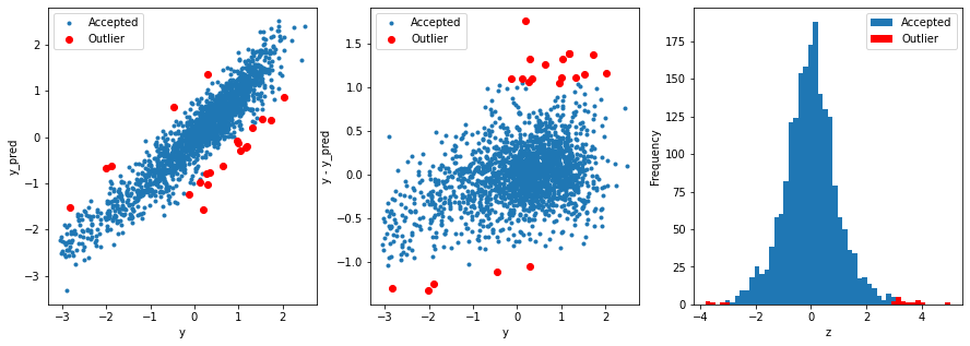

3.2 Model training

def get_trainning_data_omitoutliers():
    #获取训练数据省略异常值
    y=y_t.copy()
    X=X_t.copy()
    return X,y

def train_model(model, param_grid=[], X=[], y=[],
                splits=5, repeats=5):

    # 获取数据
    if len(y)==0:
        X,y = get_trainning_data_omitoutliers()

    # 交叉验证
    rkfold = RepeatedKFold(n_splits=splits, n_repeats=repeats)

    # 网格搜索最佳参数
    if len(param_grid)>0:
        gsearch = GridSearchCV(model, param_grid, cv=rkfold,
        scoring="neg_mean_squared_error",
        verbose=1, return_train_score=True)

        # 训练
        gsearch.fit(X,y)

        # 最好的模型
        model = gsearch.best_estimator_
        best_idx = gsearch.best_index_

        # 获取交叉验证评价指标
        grid_results = pd.DataFrame(gsearch.cv_results_)
        cv_mean = abs(grid_results.loc[best_idx,'mean_test_score'])
        cv_std = grid_results.loc[best_idx,'std_test_score']

    # 没有网格搜索
    else:
        grid_results = []
        cv_results = cross_val_score(model, X, y, scoring="neg_mean_squared_error", cv=rkfold)
        cv_mean = abs(np.mean(cv_results))
        cv_std = np.std(cv_results)

    # 合并数据
    cv_score = pd.Series({'mean':cv_mean,'std':cv_std})

    # 预测
    y_pred = model.predict(X)

    # 模型性能的统计数据
    print('----------------------')
    print(model)
    print('----------------------')
    print('score=',model.score(X,y))
    print('rmse=',rmse(y, y_pred))
    print('mse=',mse(y, y_pred))
    print('cross_val: mean=',cv_mean,', std=',cv_std)

    # 残差分析与可视化
    y_pred = pd.Series(y_pred,index=y.index)
    resid = y - y_pred
    mean_resid = resid.mean()
    std_resid = resid.std()
    z = (resid - mean_resid)/std_resid
    n_outliers = sum(abs(z)>3)
    outliers = z[abs(z)>3].index

    return model, cv_score, grid_results

from sklearn.model_selection import GridSearchCV, RepeatedKFold, cross_val_score,cross_val_predict,KFold
from sklearn.linear_model import Ridge

# 定义训练变量存储数据
opt_models = dict()
score_models = pd.DataFrame(columns=['mean','std'])
splits=5
repeats=5

model = 'Ridge'
opt_models[model] = Ridge()
alph_range = np.arange(0.25,6,0.25)
param_grid = {'alpha': alph_range}

opt_models[model],cv_score,grid_results = train_model(opt_models[model],
                    param_grid=param_grid, splits=splits, repeats=repeats)

cv_score.name = model
score_models = score_models.append(cv_score)

plt.figure()
plt.errorbar(alph_range, abs(grid_results['mean_test_score']),
        abs(grid_results['std_test_score'])/np.sqrt(splits*repeats))
plt.xlabel('alpha')
plt.ylabel('score')

Results:

Fitting 25 folds for each of 23 candidates, totalling 575 fits
----------------------
Ridge(alpha=0.25)
----------------------
score= 0.8914965873982021
rmse= 0.32638045120253134
mse= 0.1065241989271679
cross_val: mean= 0.11019851747204477 , std= 0.006413351282774973

Text(0, 0.5, 'score')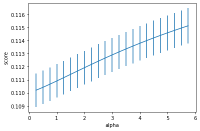

Forecasting function

# 预测函数
def model_predict(test_data,test_y=[]):
    i=0
    y_predict_total=np.zeros((test_data.shape[0],))
    for model in opt_models.keys():
        if model!="LinearSVR" and model!="KNeighbors":
            y_predict=opt_models[model].predict(test_data)
            y_predict_total+=y_predict
            i+=1
        if len(test_y)>0:
            print("{}_mse:".format(model),mean_squared_error(y_predict,test_y))

    y_predict_mean=np.round(y_predict_total/i,6)

    if len(test_y)>0:
        print("mean_mse:",mean_squared_error(y_predict_mean,test_y))
    else:
        y_predict_mean=pd.Series(y_predict_mean)
        return y_predict_mean

3.3 预测并保存结果

1 2	y_ = model_predict(test) y_.to_csv('predict.txt',header = None,index = False)

独孤诗人的学习驿站

Ensemble-Steam

1. Problem

1.1 Introduction of Background

1.2 Data source

1.3 Evaluation metrics

2. Data process

2.1 Load data

2.2 Data exploration

2.2.1 EDA

2.2.2 Dimentsionality

2.3.3 Features engineering

3. Model construction

3.1 Self definition fuction

3.2 Model training

3.3 预测并保存结果