1 Pytorch brief
1.1 Create Tensor
empty1
2import torch
x1 = torch.empty(5, 3) # 构造未初始化的矩阵rand1
x2 = torch.rand(5, 3) # 构造随机初始化的正态分布矩阵
randn1
a = torch.randn(3, 3) # [0,1]之间标准正态分布
arange1
a = torch.arange(0, 10, 2) # 0-10, steps is 2
linspace1
a = torch.linspace(0, 10, steps=5) # 0到10,分5份
zeros&ones&eye1
2
3
4
5
6x3 = torch.zeros(5, 3) # 类型为 float32
x4 = torch.zeros(5, 3, dtype=torch.long)
a = torch.ones(3, 3) # 3*3,全1矩阵
a = torch.eye(3, 3) # 3*3,对角矩阵full1
a = torch.full([2, 3], 7) # 2行3列,全是7
From datum
1
2
3x5 = torch.tensor([5.4, 3]) # 从数据创建
x6 = x5.new_ones(5, 3) # 同x5一样的数据类型
x7 = torch.randn_like(x6, dtype = torch.float) # 创建同x6一样大小的正态 TensorFrom NumPy
1
2
3
4a = np.array([2, 5.5])
print(a)
b = torch.from_numpy(a)
print(b)
1.2 Operations
1 | x = torch.rand(5, 3) |
1.2.1 Attributions
Type
1
2
3
4# 查看 x 的类型
xType1 = x.type()
xType2 = x.dtype
print('first:{}, second: {}'.format(xType1, xType2))Shape
1
2
3# 查看 Tensor 的形状
print(x.size())
print(x.shape)
1.2.2 Numerical operations
Add
1
2
3
4
5# 加法
x + y
x/y # 除法
torch.add(x, y, [out = result])
y.add_(x)in-place的运算都会以_结尾。 举例来说:x.copy_(y),x.t_(), 该操作会改变x。Metric multiple
1
2
3
4
5
6
7a = torch.ones(2, 2) * 2
b = torch.ones(2, 3)
print(torch.mm(a, b)) # 只适用于2维数组
print(a@b)
a = torch.rand(4, 32, 28, 28)
b = torch.rand(4, 32, 28, 16)
print(torch.matmul(a, b).shape) # 可以适用于多维数组,只将最后两个维度相乘mm只适用于2维数组的矩阵相乘,matmul可以适用于多维数组,只将最后两个维度相乘。Result:1
2
3
4
5tensor([[4., 4., 4.],
[4., 4., 4.]])
tensor([[4., 4., 4.],
[4., 4., 4.]])
torch.Size([4, 32, 28, 16])pow&sqrt1
2
3
4
5
6
7
8a = torch.ones(2, 2) * 2
# Pow
a.pow(2)
a**2
# sqrt
a.sqrt()
a**2Result:
1
2
3
4
5
6
7
8tensor([[4., 4.],
[4., 4.]])
tensor([[4., 4.],
[4., 4.]])
tensor([[1.4142, 1.4142],
[1.4142, 1.4142]])
tensor([[1.4142, 1.4142],
[1.4142, 1.4142]])exp&log1
2
3
4
5
6
7
# Exp
a = torch.exp(torch.ones(2, 2)) # e运算
print(a)
# Log
print(torch.log(a)) # 取对数,默认以e为底Round
1
2
3
4
5a = torch.tensor(3.14)
print(a.floor()) # 向下取整
print(a.ceil()) # 向上取整
print(a.trunc()) # 取整数部分
print(a.frac()) # 取小数部分floor:向下取整;ceil:向上取整;traunc:取整数部分:frac,取小数部分。
clampclamp可以用来限定数组的范围。1
2
3
4a = torch.rand(2, 3) * 15
print(a)
print(a.clamp(2)) # 限定最小值为2
print(a.clamp(2, 10)) # 取值范围在0-10Result:
1
2
3
4
5
6tensor([[ 0.7791, 4.7365, 4.2215],
[12.7793, 11.7283, 13.1722]])
tensor([[ 2.0000, 4.7365, 4.2215],
[12.7793, 11.7283, 13.1722]])
tensor([[ 2.0000, 4.7365, 4.2215],
[10.0000, 10.0000, 10.0000]])transpose1
2
3# 转置
y = torch.randn(2, 4)
z = y.transpose(1, 0)Switch to numpy
1
2
3
4
5
6
7# numpy 与 tensor 转换
a = torch.ones(4)
b = a.numpy() # tensor 转 numpy
c = np.ones(5)
c = torch.from_numpy(c) # numpy 转 tensor
b[2] = 3 # 浅拷贝,都会改变
# 所有CPU上的Tensor都支持转成numpy或从numpy转成TensorGet values
1
x.item() # 将单元素的 tensor 转化为 Python 数值
1.2.3 Dimensional operation
Truncate
1
2# 截取
print(x[:, 1])Concatenation:
cat1
2
3
4a = torch.rand(4, 32, 8)
b = torch.rand(5, 32, 8)
c = torch.cat([a, b], dim=0)
print(c.shape)按第
0维度进行拼接,除拼接之外的维度必须相同。Result:1
torch.Size([9, 32, 8])
stack可以利用
stack拼接,和cat命令不同,该命令会产生一个新的维度。1
2
3
4a = torch.rand(5, 32, 8)
b = torch.rand(5, 32, 8)
c = torch.stack([a, b], dim=0)
print(c.shape)产生一个新的维度,待拼接的向量维度相同。result:
1
torch.Size([2, 5, 32, 8])
split按所制定的长度对张量进行拆分。
1
2
3
4a = torch.rand(6, 32, 8)
b, c = a.split(3, dim=0) # 所给的是拆分后,每个向量的大小,指定拆分维度
print(b.shape)
print(c.shape)split所给的是拆分后,每个向量的大小,指定拆分维度。Result:1
2torch.Size([3, 32, 8])
torch.Size([3, 32, 8])chuck按所给数量进行拆分。
1
2
3
4a = torch.rand(6, 32, 8)
b, c, d = a.chuck(3, dim=0) # 所给的是拆分的个数,即拆分成多少个小,指定拆分维度
print(b.shape)
print(c.shape)所给的是拆分的个数,即拆分成多少个。Result:
1
2torch.Size([2, 32, 8])
torch.Size([2, 32, 8])reshape1
2
3
4x = torch.randn(4, 4)
y = x.view(16)
z = x.view(-1, 8) # the size -1 is inferred from other dimensions,自动计算
print(x.size(), y.size(), z.size())
1.3 GPU edition
1.3.1 Basic functions
is_available1
torch.cuda.is_avaliable() # 判断 CUDA 是否可用
device1
device = torch.device('cuda') # 将 torch 对象放入 GPU 中
Transfer tensor into CUDA
1
2
3
4
5
6
7
8
9x = torch.randn(4, 4)
y = torch.ones_like(x, device=device)
x = x.to(device)
# or just use strings ``.to("cuda")`
z = x + y
print(z)
print(z.to("cpu", torch.double))
# 先转到 cpu 中才能转numpy,因为 numpy 是在cpu上运行的tocan also change dtype together, such asz.cuda()orz.to('cuda:0'). Before turn into numpy, the data must be on cpu,becasue numpy run on cpu.Full code
1
2
3
4
5
6
7
8
9
10
11
12
13
14
15if torch.cuda.is_available():
device = torch.device("cuda")
# a CUDA device object
x = torch.randn(4, 4)
y = torch.ones_like(x, device=device)
# directly create a tensor on GPU
x = x.to(device)
# or just use strings ``.to("cuda")``
z = x + y
print(z)
print(z.to("cpu", torch.double))
# ``.to`` can also change dtype together! such as z.cuda() or z.to('cuda:0')
y.to('cpu').data.numpy()
y.cpu().data.numpy() # 先转到 cpu 中才能转numpy,因为 numpy 是在cpu上运行的
1.4 Gradient
1 | import torch |
- eg: Nural network
1 | import numpy as np |
1.5 Pytorch methods
1.5.1 Pytorch: NN
1 | import torch |
1.5.2 Pytorch: optim
1 | import torch |
1.6 Variable
1 | import torch |
2 NN
2.1 快速实现神经网络
1 | import torch |
result:
1 | Net ( |
2.2 load and save nn
- Import modules
1 | import torch |
- Generate fake data
1 | x = torch.unsqueeze(torch.linspace(-1, 1, 100), dim=1) |
- Save net
1 | def save(): |
- Reload net
1 | def restore_net(): |
- Reload net parameters
1 | def restore_params(): |
- Test
1 | # save net1 |
result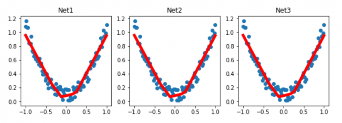
2.3 批训练
1 | import torch |
2.4 Optimizer
2.4.1 Optimization methods:
- Newton's method(牛顿法)
- Least Squares method(最小二乘法)
- Gradient Descent(梯度下降法:神经网络)
2.4.2 Gradient Descent:
- Cost Function(误差方程):
\begin{align*} Cost = (predicted - real)^2 &= (Wx - y)^2 \\ &=(W - o)^2 \end{align*}
2.4.3 Code
1 | import torch |
result:
2.5 Activation Function
1 | import torch |

sigmoid 激活函数: \sigma(x) = \frac{1}{1+e^{-x}} tanh 激活函数: tanh(x) = 2 \sigma(2x) - 1 ReLU 激活函数: ReLU(x) = max(0, x)
Softmax 激活函数: z_i \rightarrow \frac{e^{z_i}}{\sum_{j=1}^{k} e^{z_j}}
3 Examples for NN
3.1 Numpy
一个全连接ReLU神经网络,一个隐藏层,没有bias。用来从x预测y,使用L2 Loss。
- $ h = W_1 X + b_1$
- $ a = max(0, h)$
- $ y_{hat} = W_2 a + b_2$
- $ loss = (y_{hat} - y) ** 2$
Goals: 把 1000 维的向量转化维 10 维的向量
1 | import numpy as np |
3.2 Torch
- Modify according to above codes
1 | import numpy as np |
1 | import torch |
3.3 fizz_buzz demo
FizzBuzz是一个简单的小游戏。游戏规则如下:从1开始往上数数,当遇到3的倍数的时候,说fizz,当遇到5的倍数,说buzz,当遇到15的倍数,就说fizzbuzz,其他情况下则正常数数。
可以写一个简单的小程序来决定要返回正常数值还是fizz, buzz 或者 fizzbuzz
1 | import numpy as np |
定义模型的训练数据,并传入 GPU 中
1 | # hyper parameters |
定义神经网络模型
1 | model = torch.nn.Sequential( |
- 为了让我们的模型学会FizzBuzz这个游戏,我们需要定义一个损失函数,和一个优化算法。
- 这个优化算法会不断优化(降低)损失函数,使得模型的在该任务上取得尽可能低的损失值。
- 损失值低往往表示我们的模型表现好,损失值高表示我们的模型表现差。
- 由于FizzBuzz游戏本质上是一个分类问题,我们选用Cross Entropyy Loss函数。
- 优化函数我们选用Stochastic Gradient Descent。
1 | # loss function |
训练模型
1 | BATCH_SIZE = 128 |
最后用训练好的模型尝试在 1-100 中玩 FizzBuzz 邮箱
1 | testX = torch.Tensor([binary_encode(i, NUM_DIGITS) for i in range(1, 101)]) |
3.3.1 Full code
1 | import numpy as np |