1 Installing scikit-learn
Windows
1
pip install -U scikit-learn
macOS
1
pip install -U scikit-learn
Linux
1
pip3 install -U scikit-learn
Check installation:
1 | pip show scikit-learn |
See more about scikit-learn via clicking here.
2 General study mode
Steps:
- Load datas
- Split datas into two part: train and test part
- Training model
- Testing and evaluating model
1 | # instance for iris |
Result:
1 | [1 1 0 0 0 2 2 0 0 2 1 0 2 0 0 2 2 2 0 1 2 1 0 1 0 1 2 2 1 0 2 0 1 1 0 0 0 0 1 2 1 2 0 2 2] |
3 Sklearn.datasets
3.1 Generate regressiong datas
1 | # instance for making datasets |
Result: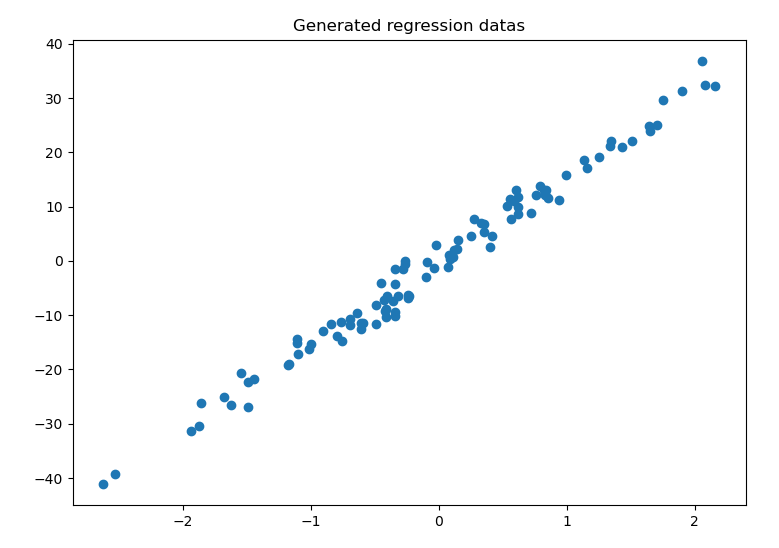
3.2 Load datasets of Linear Regression
1 | # instance for loading boston datasets |
Result:
1 | [24. 21.6 34.7 33.4] |
3.3 Normalization
Demo
1
2
3
4
5
6
7
8
9
10
11
12
13
14from sklearn import preprocessing
import numpy as np
from sklearn.model_selection import train_test_split
# cross_validation 更新为 model_selection
from sklearn.datasets.samples_generator import make_classification
from sklearn.svm import SVC
import matplotlib.pyplot as plt
a = np.array([[10, 2.7, 3.6],
[-100, 5, 2],
[120, 20, 40]], dtype = np.float64)
print(a)
print(preprocessing.scale(a)) # normalizationResult:
1
2
3
4
5
6[[ 10. 2.7 3.6]
[-100. 5. 2. ]
[ 120. 20. 40. ]]
[[ 0. -0.85170713 -0.66102858]
[-1.22474487 -0.55187146 -0.75220493]
[ 1.22474487 1.40357859 1.41323351]]Comparison of accuracy before and after normalization
1
2
3
4
5
6
7
8
9
10
11
12
13
14from sklearn import preprocessing
import numpy as np
from sklearn.model_selection import train_test_split
# cross_validation 更新为 model_selection
from sklearn.datasets.samples_generator import make_classification
from sklearn.svm import SVC
import matplotlib.pyplot as plt
X, y = make_classification(n_samples = 300, n_features = 2, n_redundant = 0,n_informative = 2, random_state = 22, n_clusters_per_class = 1, scale = 100)
# random_state: 固定随机数
plt.scatter(X[:, 0], X[:, 1], c = y)
plt.title('Classification samples')
plt.show() #Plot the generated samples:
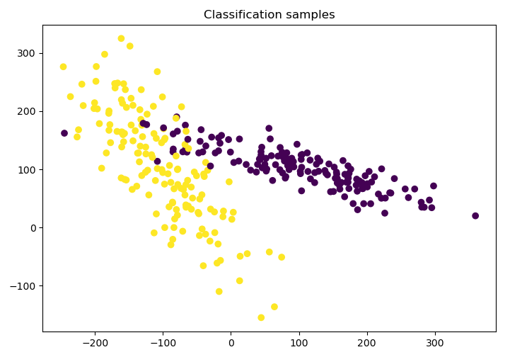
fig. 3-2 Samples
1
2
3
4
5
6
7
8
9
10X_train, X_test, y_train, y_test = train_test_split(X, y ,test_size = .3)
clf = SVC()
clf.fit(X_train, y_train)
print(clf.score(X_test, y_test))
X = preprocessing.scale(X) # normalization
X_train, X_test, y_train, y_test = train_test_split(X, y ,test_size = .3)
clf = SVC()
clf.fit(X_train, y_train)
print(clf.score(X_test, y_test))Result:
1
20.9111111111111111
0.9555555555555556
4 Model features and attributes
4.1 Basic parameters
1 | from sklearn import datasets |
Result:
1 | [24. 21.6 34.7 33.4] |
4.2 Cross validation
Evaluate the NN
1
2
3
4
5
6
7
8
9
10
11
12
13
14
15
16
17from sklearn.datasets import load_iris
from sklearn.model_selection import train_test_split
from sklearn.neighbors import KNeighborsClassifier
from sklearn.model_selection import cross_val_score
iris = load_iris()
X = iris.data
y = iris.target
X_train, X_test, y_train, y_test = train_test_split(X, y, random_state = 4)
knn = KNeighborsClassifier(n_neighbors = 5)
# knn.fit(X_train, y_train)
# print(knn.score(X_test, y_test))
scores = cross_val_score(knn, X, y, cv = 5, scoring = 'accuracy') # 将test进行5次划分
print(scores.mean()) # 取平均值Result:
1
0.9733333333333334
Cross validation
1
2
3
4
5
6
7
8
9
10
11
12
13
14
15
16
17
18
19
20
21
22
23
24
25from __future__ import print_function
from sklearn.model_selection import learning_curve
from sklearn.datasets import load_digits
from sklearn.svm import SVC
import matplotlib.pyplot as plt
import numpy as np
digits = load_digits()
X = digits.data
y = digits.target
train_sizes, train_loss, test_loss= learning_curve( SVC(gamma=0.01), X, y, cv=10, scoring='neg_mean_squared_error', train_sizes=[0.1, 0.25, 0.5, 0.75, 1])
# 'neg_mean_squared_error' 非 'mean_squared_error'
train_loss_mean = -np.mean(train_loss, axis=1)
test_loss_mean = -np.mean(test_loss, axis=1)
plt.plot(train_sizes, train_loss_mean, 'o-', color="r",
label="Training")
plt.plot(train_sizes, test_loss_mean, 'o-', color="g",
label="Cross-validation")
plt.xlabel("Training examples")
plt.ylabel("Loss")
plt.legend(loc="best")
plt.show()Result:
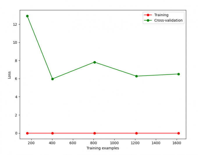
fig 4-1 Vross-validation
Adjustment parameter-1
1
2
3
4
5
6
7
8
9
10
11
12
13
14
15
16
17
18
19
20
21
22
23
24
25
26
27
28
29
30
31from __future__ import print_function
from sklearn.datasets import load_iris
from sklearn.model_selection import train_test_split
from sklearn.neighbors import KNeighborsClassifier
iris = load_iris()
X = iris.data
y = iris.target
# test train split #
X_train, X_test, y_train, y_test = train_test_split(X, y, random_state=4)
knn = KNeighborsClassifier(n_neighbors=5)
knn.fit(X_train, y_train)
y_pred = knn.predict(X_test)
print(knn.score(X_test, y_test))
# this is how to use cross_val_score to choose model and configs #
from sklearn.model_selection import cross_val_score
import matplotlib.pyplot as plt
k_range = range(1, 31)
k_scores = []
for k in k_range:
knn = KNeighborsClassifier(n_neighbors=k)
## loss = -cross_val_score(knn, X, y, cv=10, scoring='mean_squared_error') # for regression
scores = cross_val_score(knn, X, y, cv=10, scoring='accuracy') # for classification
k_scores.append(scores.mean())
plt.plot(k_range, k_scores)
plt.xlabel('Value of K for KNN')
plt.ylabel('Cross-Validated Accuracy')
plt.show()Result:

fig. 4-2 Adjustment parameters
Adjustment parameter-2
1
2
3
4
5
6
7
8
9
10
11
12
13
14
15
16
17
18
19
20
21
22
23
24
25
26
27from __future__ import print_function
from sklearn.model_selection import validation_curve
from sklearn.datasets import load_digits
from sklearn.svm import SVC
import matplotlib.pyplot as plt
import numpy as np
digits = load_digits()
X = digits.data
y = digits.target
param_range = np.logspace(-6, -2.3, 5)
train_loss, test_loss = validation_curve(
SVC(), X, y, param_name='gamma', param_range=param_range, cv=10,
scoring= 'neg_mean_squared_error')
train_loss_mean = -np.mean(train_loss, axis=1)
test_loss_mean = -np.mean(test_loss, axis=1)
plt.plot(param_range, train_loss_mean, 'o-', color="r",
label="Training")
plt.plot(param_range, test_loss_mean, 'o-', color="g",
label="Cross-validation")
plt.xlabel("gamma")
plt.ylabel("Loss")
plt.title('Overfitting problem')
plt.legend(loc="best")
plt.show()Result:

fig 4-3 Adjustment parameters
4.3 Transform target in regression model
将原始数据转化为分类模式,可以有效地提高预测的精度,效果如下:
1 | import numpy as np |
Result:
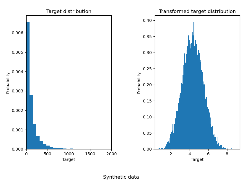
然后,再来测试其对预测精度的影响:
1 | X_train, X_test, y_train, y_test = train_test_split(X, y, random_state=0) |

从结果可以看出,经过预处理转化后的数据集能有效地提高预测的精度,降低
MAE 的值。
5 Save model
Train model
1 | from __future__ import print_function |
Then, we can use two methods to save our trained models:
pickle
1
2
3
4
5
6
7
8import pickle
# Save
with open('save/clf.pickle', 'wb') as f:
pickle.dump(clf, f)
# Restore
with open('save/clf.pickle', 'rb') as f:
clf2 = pickle.load(f)
print(clf2.predict(X[0:1]))joblib
1
2
3
4
5
6import joblib
# Save
joblib.dump(clf, './save/clf.pkl')
# restore
clf3 = joblib.load('save/clf.pkl')
print(clf3.predict(X[0:1]))